Penny Pinching: Statistical Treatment of Data
By: Julie Wilhelmsen
Objective:
The objective of experiment one is to see if the year a penny is produced in mint, relates to the weight of the penny. Each lab group had a set of 20 pennies, in which we collected the weight and the year of each penny. The information obtained from each lab group will help us create some statistical data. By using different calculations, I will be able to determine if there is a relation between a penny’s weight and year minted. The calculations I will use to do this are: mean, standard deviation, Q-test, and t-test. I predict that pennies that are newly produced will weigh less than pennies produced many years ago.
Data:
Table 1: Individual Lab Group Data
|
Penny # |
Year |
Mass (g) |
|
1 |
1980 |
3.0841 |
|
2 |
2005 |
2.4948 |
|
3 |
1982 |
3.0996 |
|
4 |
1996 |
2.5038 |
|
5 |
1993 |
2.4829 |
|
6 |
1988 |
2.4724 |
|
7 |
1984 |
2.5723 |
|
8 |
1995 |
2.5191 |
|
9 |
1990 |
2.5269 |
|
10 |
1979 |
3.1068 |
|
11 |
1999 |
2.4890 |
|
12 |
1995 |
2.4901 |
|
13 |
1984 |
2.5202 |
|
14 |
1988 |
2.5154 |
|
15 |
1983 |
2.5108 |
|
16 |
1974 |
3.0823 |
|
17 |
1991 |
2.4502 |
|
18 |
1993 |
2.4807 |
|
19 |
1985 |
2.4657 |
|
20 |
1963 |
3.0910 |
Table 2: Class Data
|
Penny # |
Year |
Mass (g) |
Penny # |
Year |
Mass (g) |
|
1 |
1988 |
2.4444 |
41 |
1994 |
2.4624 |
|
2 |
1993 |
2.5002 |
42 |
1996 |
2.4743 |
|
3 |
1990 |
2.4990 |
43 |
1991 |
2.5226 |
|
4 |
1990 |
2.4711 |
44 |
1979 |
3.0753 |
|
5 |
1959 |
3.0603 |
45 |
1968 |
3.0454 |
|
6 |
1994 |
2.4732 |
46 |
1990 |
2.4991 |
|
7 |
1993 |
2.4857 |
47 |
1995 |
2.4516 |
|
8 |
2001 |
2.4843 |
48 |
1985 |
2.5118 |
|
9 |
1993 |
2.5222 |
49 |
2005 |
2.5108 |
|
10 |
2001 |
2.5035 |
50 |
1969 |
3.0703 |
|
11 |
1982 |
3.1035 |
51 |
1972 |
3.0694 |
|
12 |
1974 |
3.1047 |
52 |
1984 |
2.483 |
|
13 |
1989 |
2.5413 |
53 |
1996 |
2.4724 |
|
14 |
1989 |
2.4786 |
54 |
1982 |
3.116 |
|
15 |
1986 |
2.4923 |
55 |
1982 |
3.1009 |
|
16 |
1982 |
3.0563 |
56 |
1987 |
2.5218 |
|
17 |
1988 |
2.4533 |
57 |
1999 |
2.4892 |
|
18 |
1973 |
3.1142 |
58 |
1988 |
2.4492 |
|
19 |
1964 |
3.1085 |
59 |
1987 |
2.5223 |
|
20 |
1972 |
3.1025 |
60 |
1994 |
2.5136 |
|
21 |
1981 |
3.0091 |
61 |
1979 |
3.1048 |
|
22 |
1991 |
2.5374 |
62 |
1988 |
2.5082 |
|
23 |
1986 |
2.5418 |
63 |
1999 |
2.5111 |
|
24 |
1978 |
3.1921 |
64 |
1995 |
2.4893 |
|
25 |
2006 |
2.4812 |
65 |
1970 |
3.1001 |
|
26 |
1982 |
3.1121 |
66 |
2005 |
2.4979 |
|
27 |
1980 |
3.1286 |
67 |
1996 |
2.5063 |
|
28 |
1975 |
3.1243 |
68 |
1977 |
3.1096 |
|
29 |
1996 |
2.5083 |
69 |
1989 |
2.4948 |
|
30 |
2005 |
2.5084 |
70 |
1975 |
3.1283 |
|
31 |
1995 |
2.5006 |
71 |
1983 |
2.5272 |
|
32 |
1978 |
3.1169 |
72 |
1973 |
3.0811 |
|
33 |
1982 |
3.096 |
73 |
1995 |
2.4991 |
|
34 |
1959 |
3.1042 |
74 |
1978 |
3.1055 |
|
35 |
1980 |
3.0782 |
75 |
1989 |
2.5331 |
|
36 |
1989 |
2.4955 |
76 |
1982 |
3.1122 |
|
37 |
1990 |
2.5159 |
77 |
1986 |
2.4782 |
|
39 |
1993 |
2.5036 |
79 |
2003 |
2.5107 |
|
40 |
2001 |
2.4992 |
80 |
1994 |
2.517 |
|
Penny # |
Year |
Mass (g) |
Penny # |
Year |
Mass (g) |
|
81 |
1987 |
2.4966 |
121 |
1994 |
2.4963 |
|
82 |
1984 |
2.5722 |
122 |
1992 |
2.5107 |
|
83 |
1990 |
2.5288 |
123 |
1977 |
3.1174 |
|
84 |
1984 |
2.5001 |
124 |
2003 |
2.4819 |
|
85 |
1973 |
3.0682 |
125 |
1968 |
3.0723 |
|
86 |
1991 |
2.5163 |
126 |
2000 |
2.4884 |
|
87 |
2000 |
2.4757 |
127 |
1996 |
2.4955 |
|
88 |
1983 |
2.5606 |
128 |
1998 |
2.4758 |
|
89 |
1990 |
2.5261 |
129 |
1974 |
3.0957 |
|
90 |
1988 |
2.4743 |
130 |
2001 |
2.4866 |
|
91 |
1990 |
2.4639 |
131 |
1982 |
3.115 |
|
92 |
2001 |
2.5159 |
132 |
1979 |
3.0664 |
|
93 |
1986 |
2.5069 |
133 |
1988 |
2.9095 |
|
94 |
1989 |
2.4943 |
134 |
1992 |
2.4875 |
|
95 |
1996 |
2.4903 |
135 |
1975 |
3.1285 |
|
96 |
1975 |
3.1156 |
136 |
1984 |
2.5368 |
|
97 |
1986 |
2.5199 |
137 |
1963 |
3.0583 |
|
98 |
1980 |
3.1549 |
138 |
1994 |
2.5095 |
|
99 |
1990 |
2.4611 |
139 |
1998 |
2.5221 |
|
100 |
1997 |
2.5042 |
140 |
1980 |
3.0947 |
|
101 |
1980 |
3.0841 |
141 |
1994 |
2.4963 |
|
102 |
2005 |
2.4948 |
142 |
1992 |
2.5107 |
|
103 |
1982 |
3.0996 |
143 |
1977 |
3.1174 |
|
104 |
1996 |
2.5038 |
144 |
2003 |
2.4819 |
|
105 |
1993 |
2.4829 |
145 |
1968 |
3.0723 |
|
106 |
1988 |
2.4724 |
146 |
2000 |
2.4884 |
|
107 |
1984 |
2.5723 |
147 |
1996 |
2.4955 |
|
108 |
1995 |
2.5191 |
148 |
1998 |
2.4758 |
|
109 |
1990 |
2.5269 |
149 |
1974 |
3.0957 |
|
110 |
1979 |
3.1068 |
150 |
2001 |
2.4866 |
|
111 |
1999 |
2.489 |
151 |
1982 |
2.115 |
|
112 |
1995 |
2.4901 |
152 |
1979 |
3.0664 |
|
113 |
1984 |
2.5202 |
153 |
1988 |
2.5095 |
|
114 |
1988 |
2.5154 |
154 |
1992 |
2.4875 |
|
115 |
1983 |
2.5108 |
155 |
1975 |
2.1285 |
|
116 |
1974 |
3.0823 |
156 |
1984 |
2.5368 |
|
117 |
1991 |
2.4502 |
157 |
1963 |
3.0583 |
|
119 |
1985 |
2.4657 |
159 |
1998 |
2.5221 |
|
120 |
1963 |
3.091 |
160 |
1980 |
3.0947 |
Calculations and Graphs:
Constants Used in Calculations:
Qcrit (n=20) at 90% confidence = 0.300
This value was found on “Q” test table provided by Dr. Schug. The table was adapted from D.B. Rorabache, Anal. Chem., 63 (1981) 139.
ttable (DOF = ∞) at 99% confidence level = 2.576
This value was found on Values of Student’s t Table provided by Dr. Schug. The table was originally found in Quantitative Chemical Analysis, Seventh Edition ©2007 W.H. Freeman and Company.
Q-Test Calculations for Individual Data
Qcalc = Gap/Range
Gap (low) = 2.4657 – 2.4502 = 0.0155g
Gap (high) = 3.1068 – 3.0996 = 0.007g
Range (high-low) = 3.1068 – 2.4502 = 0.6566g
Qcalc(low) = 0.0155/0.6566 = 0.0236
Qcalc(low) < Qcrit
Qcalc(high) = 0.007/0.6566 = 0.11
Qcalc(high) < Qcrit
Q calculated in both cases (high and low) is less than Q critical (table), so we retain both values.
Mean of individual data=2.6479 g
Mean = ∑xi/n
∑ xi = sum of measured values
n = number of measurements
Standard deviation (s)=0.2648 g
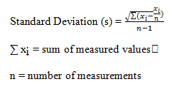
Table 3: Low and High Frequency Table for Class Data
| Range (g) low distribution | # of Pennies | Range (g) high distribution | # of Pennies |
| 2.100 to 2.325 |
2 |
2.800 to 2.825 |
0 |
| 2.325 to 2.350 |
0 |
2.825 to 2.850 |
0 |
| 2.350 to 2.375 |
0 |
2.850 to 2.875 |
0 |
| 2.375 to 2.400 |
0 |
2.875 to 2.900 |
0 |
| 2.400 to 2.425 |
0 |
2.900 to 2.925 |
1 |
| 2.400 to 2.425 |
0 |
2.900 to 2.925 |
1 |
| 2.425 to 2.450 |
2 |
2.925 to 2.950 |
0 |
| 2.450 to 2.475 |
13 |
2.950 to 2.975 |
0 |
| 2.475 to 2.500 |
40 |
2.975 to 3.000 |
0 |
| 2.500 to 2.525 |
37 |
3.000 to 3.025 |
1 |
| 2.525 to 2.550 |
10 |
3.025 to 3.050 |
1 |
| 2.550 to 2.575 |
3 |
3.050 to 3.075 |
11 |
| 2.575 to 2.600 |
0 |
3.075 to 3.100 |
13 |
| 2.600 to 2.625 |
0 |
3.100 to 3.125 |
21 |
| 2.625 to 2.650 |
0 |
3.125 to 3.150 |
3 |
| 2.650 to 2.675 |
0 |
3.150 to 3.175 |
1 |
| 2.675 to 2.700 |
0 |
3.175 to 3.200 |
1 |
| 2.700 to 2.725 |
0 |
3.200 to 3.225 |
0 |
| 2.725 to 2.750 |
0 |
3.225 to 3.250 |
0 |
| 2.7250 to 2.775 |
0 |
3.250 to 3.275 |
0 |
| 2.775 to 2.800 |
0 |
3.275 to 3.300 |
0 |
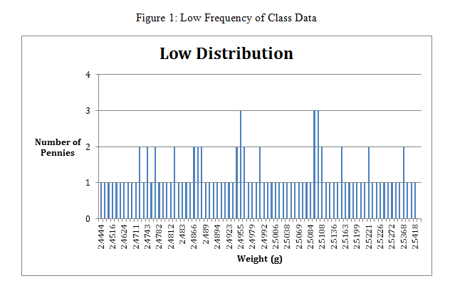
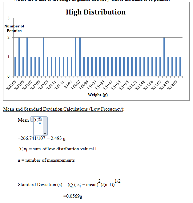
Figure 2: High Frequency of Class Data
Where the x-axis is the range in grams, and the y-axis is the number of pennies.
Individual Data
While performing the experiment, it became evident that there was a range of weights that can be expressed on table 1. When we calculated the Q-test, it revealed that the two highest and two lowest values were not outliers. By performing these calculations we can visibly see a difference between the highest and lowest values. After dividing these values by the range, we calculate the critical value. After calculating the critical value, it was determined that no values should be disregarded because the calculated Q-test value was less than the provided critical value.
The mean of pennies weights was 2.6479. This means that the masses were relatively close. The mean is the average weight of all the pennies in the experiment. The standard deviation is calculated to show how many of the pennies fell near the mean weight for the penny. The standard deviation was 0.2648. The standard deviation being low means that most of the pennies masses were close to the mean.
Results
After reviewing the complied data from the class, it was evident that there were a large majority of the masses were around 3 grams. If you look at the histograms ( Figure 1 and Figure 2), you can see the frequency distribution for the masses of the pennies. In order to tell completely analyze the data, more tests and calculation were done.
The mean and the standard deviation of the low frequency distribution of penny’s weights were calculated. The mean of the low frequency was calculated to be 2.493g and the standard deviation to be 0.0569g. The standard deviation being low means that more pennies were weighed, in which we were able to obtain more data. This means that because there is more data, the mean and the standard deviation are closer to the actual value.
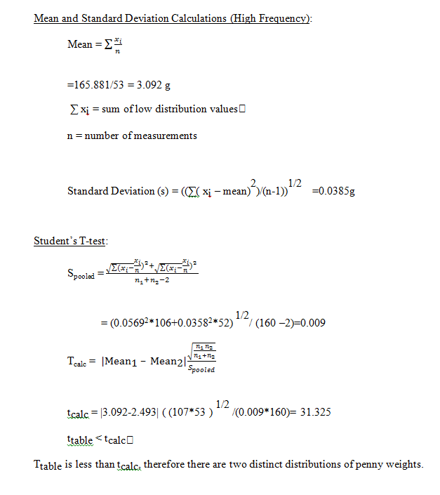
The mean and the standard deviation for the high frequency distribution of penny’s weights were also calculated. The mean calculated was 3.092g and the standard deviation was 0.0385g. This puts the measurements in the range of 3.0535g to 3.1305g for the high frequency.
By calculating the two frequencies, it became evident that a T-test needed to be done to verify the data. First, the pooled standard deviation (S pool) is calculated. This was needed to plug into the T calc equation. After calculating a T-value, it was compared that value to the t-table value. Because T table was less than T calc at a 99% confidence, it can be assumed that there are two distinct distributions.
Conclusions:
It can be concluded that there is a relation between the pennies masses and the year minted. I predicted that pennies that are more newly produced would weigh less than pennies produced many years ago. This seemed to hold true while analyzing our data.
By looking at both individual and class datum, we can see two distinct average masses. In both, individual data and class data the mean was calculated, along with standard deviation, to indicate how far the measurements range is. Because the individual data’s standard deviation was higher this means that it isn’t as precise, due to less measurements. By adding more measurements, the standard deviation decreased. When I calculated the Q-test it led me to believe that no values were to be discarded in the datum. The reason some of the penny’s weights were so far off from the mean is most likely because of being measured incorrectly (human error).
I was able to conclude that the majority of that data is closer to the mean in the class data than in comparison to the individual datum. This is evident because you can slightly tell there is a Gaussian distribution in figures 1 and 2. This just shows that the measurements were replicated enough times to account for a random error, if any. When I compared the t-test datum more closely, I was able to conclude that there are two distinct distributions. The confidence interval was 99%.
