Raman Spectroscopy of Benzene
Abstract
Introduction:
In Raman Spectroscopy is a powerful technique to analyze different compounds and has a variety of applications. The theory behind this is derived from the Raman Effect (1)
The Raman effect refers to the scattering of light after it interacts with a molecule. When a molecule interacts with light, there is a change in the intensity of the light between the incoming and outgoing intensities. This can be described via the Beer Lambert law in equation 1. (2)
I = I*e^(-Ecd) (1)
I refers to the outgoing intensity, I0, is the incoming intensity of light, is the molecular absorption constant, c is the concentration of the sample, and d is path length of the cuvette (2).
Only 1 in 107 molecules participate in the Raman effect. The effect refers to the excitation of the molecule to go to an excited, virtual state. A virtual state refers to state that a molecule cannot excite to without the incident radiation, rather it is a linear combinations of real states Furthermore, it is not a vibrational or electronic state as it is not a solution of the Schrodinger Equation, Equation 2 (2).
(2)
Where …
The advantage of accessing the virtual state is that states that were previously not available from the initial state are now available. It serves as an intermediate to access states that were previously considered forbidden due to the selection rules. Through these intermediate, the energy to go form the initial vibrational level to the final one can be calculated (2)
During the experiment, once the laser light hits the molecule, the outgoing light is perpendicular to the incident beam. There are two types of scattering, Raleigh & Raman. Raleigh scattering has the same frequency as original light source, denoted as v0. Raman scattering on the other hand, is much weaker in comparison, about 10-5 of the incident light. The frequencies of the Raman scattered light are (v0 + vm) and (v0 – vm), where vm is referred as the vibrational frequency of the molecule. Each of these frequencies correspond to what is known as Anti Stokes and Stokes shifted frequency respectively. This experiment focuses on the strokes shifted frequency. Since it is more intense than the anti strokes frequency, it is commonly more measured.
The theory of Raman Scattering revolves around the following. Equation 3 represents the electric field as a function of time
(3)
is the electric field amplitude, and is the incident light. Multiplying each side of equation 3 by , the polarizibility constant forms equation 4, which demonstrates the electric dipole moment P of a molecule as a function of time. In IR, the change in dipole moment causes the transitions while in Raman spectroscopy, the change in polarizability causes the transitions. (2)
(4)
The frequency, vm, at which a molecule vibrates, is also related to the nuclear displacement q, as shown in equation 4, which parallels equation 5.
(5)
In equation 5, vm, refers to the vibrational amplitude of the mth vibrational mode. is a function of , given for small amplitude vibrations only, demonstrated in equation 6.
is the polarizibility at the equilibrium positon,. Refers to the rate of change of the polarziability in respect to the change of q at that equilibrium position. If the variation of the polarizability is only caused by the displacement along the mth coordinate, equatiosn 6. And 4 can be combined to generate equation 7.
Electric fields distorts a molecule as the nucleus will be attracted toward the negative end and the elctrons toward the positive end. While equation 3 describes this separation, this model does not accuarelty describe the situation. To describe this model, Equation 4 must be extended to all 3 dimensions.
Since the centripetal and attraction force is equivalent, the term, can be isolated and substituted into the kinetic energy equation to reduce equation 4 as follows (3)
(7)
(16)
Equation 1 can be applied to other Hydrogenic atoms, such as He+ and Li2+ since they both only have 1 electron (2). However, since they have more number of protons, holding the electron closer to the nucleus (4). As a result, the nuclear charge constant Z is introduced to account for this effect (4)
(17)
The overall goal of this experiment is use the visible spectra from both Hydrogen and Helium to calculate the ionization energy of Helium. The transition of energy states from n2 to n1, where n1=2 will be used since these transitions tend to be visible(Figure 1).
These arising spectral lines from the transitions is known as the balmer series. The Hydrogen emissions lines are used as calibration to determine the emission lines in the Helium spectrum. This data can then be used to calculate the Zeff for Helium, which can be used to determine the transition energy between n=2 state and infinity. This energy can then be used to determine the ionization energy (2).
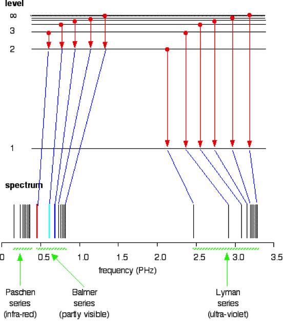
Figure 1: Spectrum of various series and their transition (5)
Spectroscopy can also be used to for fluorescence analysis. Wirz et all used a monochromator to measure the intensity of the emitted light of four antihistamines. They wanted to observe the effect on halide ions and different ligands would have on the emitted intensity (6)
Radicals play an important role in various mechanisms. Yoon and Lee analyze radicals of Benzyl type radicals by using a monochromator to obtain a vibrational emission spectrum. They used this spectrum to identify to different isomers (7)
Methods
Before the start of the experiment, care was taken to ensure the lights in the room were turned off to prevent interference. A Hydrogen discharge tube (Fisher Spectrum Tubes) was placed into a hand-tuned spectrograph, in the entrance slit of the hand tuned Spectrograph (Gaertner Scientifci corporation, Chicago serial no. 1060AW). The gas power tube used was Spectrum Tube power supply model SP200, of 5000v technic products. A knob on the side of the instrument was rotated to go through the entire visible spectrum. As spectral line became more visible, they were centered so that the “x” from the lens was perfectly in the middle (2)
The resolution was improved by using the fine course nob. The wavelengths that corresponded to each spectral line were then recorded. The process was then repeated with a He discharge tube (Fisher Spectrum tubes). Analysis was then done with Microsoft Excel to determine the ionization constant of He based off this data (2)
The next part of the experiment, an Ocean Optics USB4000 was used to analyze the emission lines of Hydrogen and Helium. The polychromator analyzed the Hydrogen tube twice, under two different integration times. Having the slower speed, allows for more light intensity but as a result, the peaks were off the graph. This was conversely true for the faster speed. The process was then repeated for Helium. The data from these experiment was exported using the Ocean Optics SpectraSuite software to export as data that encompassed the wavelengths, and corresponding transmittance. MathCad Prime 1.0 was used to read these files to obtain the wavelengths corresponding to the emission lines. Microsoft Excel was then used to analysis the data as before to determine the Zeff and the ionization energy (2)
Results & Discussion:
Hand Tuned Spectrograph:
The observed emissions from the hand tuned spectrograph hydrogen are as follows (Table 1).
Table 1: Observed wavelengths for Hydrogen Emission Lines under the monochromator
|
Observed wavelengths (nm) |
|
651.2 ± 0.1 |
|
486.6 ± 0.1 |
|
435.4 ± 0.1 |
|
411.3 ± 0.1 |
The theoretical wavelengths for the emissions lines were calculated by the Rydberg equation, where n1=2 and n2 was set to 3, 4, 5, and 6. The theoretical and experimental wavelengths were then converted to frequencies and graphed (Figure 2 ). The linear equation arising from this graph was used as calibration for the Helium emission lines. The observed Helium emission lines need to be calibrated since the hand tuned graph is not that accurate (2).
Table 2 reflects the observed emission lines for Helium(Table 2)
These values were then calibrated using the equation from figure z1 to get the adjusted wavelengths and frequencies for the Helium emission lines. A 13×13 of the adjusted frequencies for He was made to get a table of transition ratios. These ratios were then compared to the followed hydrogen ratios (Table 3). These ratios should all be in one row or column(8)
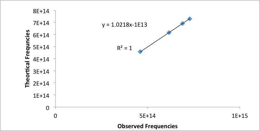
Figure 2: Graph of theoretical frequencies versus the observed frequencies for Hydrogen emission lines.
Table 2: Observed wavelengths for helium emission lines under the monochromator
|
Observed wavelengths For He (nm) |
|
700.0 ± 0.1 |
|
663.0 ± 0.1 |
|
585.8 ± 0.1 |
|
505.1 ± 0.1 |
|
501.9 ± 0.1 |
|
492.7 ± 0.1 |
|
472.3 ± 0.1 |
|
463.9 ± 0.1 |
|
448.6 ± 0.1 |
|
440.1 ± 0.1 |
|
413.9 ± 0.1 |
|
404.4 ± 0.1 |
|
390.4 ± 0.1 |
Table 3: Hydrogen Transition Ratios
|
Transition |
Transition Ratio |
| n3 —> n2 |
1 |
| n4 —> n2 |
1.35 |
| n5 —> n2 |
1.512 |
| n6 —> n2 |
1.6 |
The four transitions were then assigned to the four Helium transition ratios that best matched the hydrogen ones (Table 3, Table 4).
Table 4: Assigned helium wavelengths to balmer series transitions
|
Transition |
Wavelength (nm) |
| n3 —> n2 |
668 ± 4 |
| n4 —> n2 |
493 ± 2 |
| n5 —> n2 |
439 ± 2 |
| n6 —> n2 |
413 ± 2 |
These wavelengths were then converted to frequencies, and then graphed against the theoretical ratios based off the Rydberg equation (Figure 3). This was used to obtain the slope of this equation which was used to determine the Zeff.
The Zeff was calculated to be .995 ± 0.003. This was then used to calculate transition energy from the n=2 state to infinity. This values was then to calculate the transition energy from the state n=2 to infinity. This value was then used to calculate the ionization energy of helium to be 198300 ± 100 cm-1
Ocean Optics Polychromator:
For the Polychromator, two scans of each discharge tube, Hydrogen and Helium, under different integration times were performed. Mathcad was used to determine the wavelengths that corresponded to each peak. The average of each pair of corresponding peaks in the scans was taken. For hydrogen, the following wavelengths corresponded to the transition peaks (Table 5).
Table 5: Observed wavelengths for Hydrogen Emission Lines under the polychromator
|
Observed wavelengths (nm) |
|
655.79 ± 0.01 |
|
487.52 ± 0.01 |
|
434.23 ± 0.01 |
|
420.21 ± 0.01 |
The observed frequencies was then graphed against the theoretical frequencies (Figure 3). This was used to calibrate the Helium emission lines.
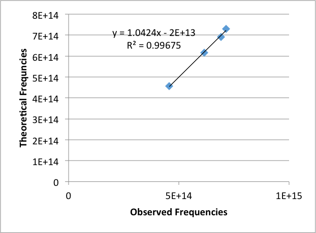
Figure 3: Graph of theoretical frequencies versus the observed frequencies for Hydrogen emission lines.
Table 6 reflects the observed Helium wavelengths (Table 6)
These values were then calibrated using the equation from figure 3 (Figure 3). Just as for the analysis for the monochromator, a table of these adjusted frequencies were used to populate a table of ratios between transitions. Using this table, four transitions were then assigned to the four of the Helium wavelengths by determine which ratios best matched the ratios for the transitions from Table 3(Table 3, Table 7). These ratios should all be in one row or column (8)
These adjusted wavelengths were converted to frequncies and then graphed versus the transition
ratio values in order to obtain the Zeff value (Figure 5)
The slope was of this line was used to calculate the Zeff of Helium to be 1.003 ± .005. This was then used to calculate transition energy from the n=2 state to infinity. This value was then used to calculate the ionization energy of helium to 198700 ± 400 cm-1
Table 6: Observed wavelengths for helium emission lines under the Polychromator
|
Observed Helium Wavelengths |
|
726.98± .01 |
|
704.86 ± .01 |
|
668.41 ± .01 |
|
589.88 ± .01 |
|
502.94 ± .01 |
|
493.12 ± .01 |
|
470.70- ± .01 |
|
446.85 ± .01 |
|
414.59 ± .01 |
|
404.78 ± .01 |
|
387.96 ± .01 |
Table 7: Assigned helium wavelengths to balmer series transitions
|
Transition |
Wavelength |
| n3 —> n2 |
672± 5 |
| n4 —> n2 |
490 ± 3 |
| n5 —> n2 |
442 ± 3 |
| n6 —> n2 |
399 ± 2 |
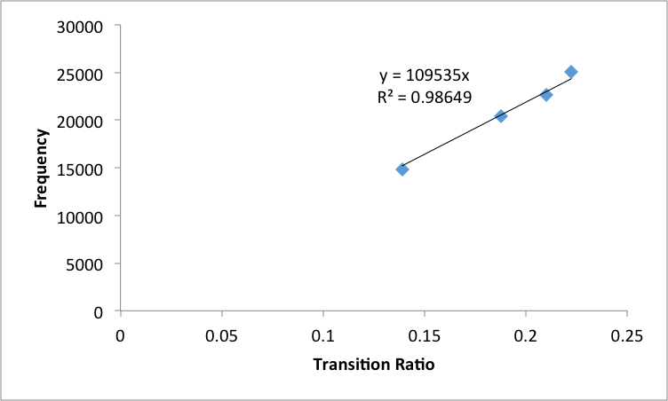
Figure 5: Adjusted Frequencies of emission lines by polychromator of Helium versus transition ratios
Error Analysis:
The literature value for the Ionization Energy of Helium is reported to be 198310.74 +.02 cm-1 (8). For the monochromator, there is 68% certainty that the literature value falls within 1 standard deviation of the experimental value .The percent error between the theoretical and calculated Ionization energy was .003%.
For the polychromator, there is 68% certainty that the literature value falls within 1 standard deviation of the experimental value. The percent error between the theoretical and calculated Ionization energy was .2%.
It is evident that the there was a larger percent error for the polychromator. This can be attribuited that since the polychromator uses an array to measure all the wavelengths simuatlensouly, there is less resolution, so the values are less accurate. While the monochromator uses a narrow range of wavelengths. As a result , it takes longer, but the resolution is greater and thus the monochromator instrument will have more accurate values (when calibrated). (9)
The method for determining ionization energy in this experiment shall work for any two-electron atom such as Li+. Since Li+ would have the same electron configuration as He and the excited electron would behave similar to a excited hydrogenic atom(1). The only difference is that Li\+ would have an additional proton, which would increase the shielding effect (4).
This could introduce a higher inaccuracy in calculating the ionization energy
For atoms with more than two electrons, this method would not work. These atoms will have large atomic radii, and a result, the electrons will be farther from the nucleus (1) . Furthermore, the additional electron will have its own magnetic moment, which will result in energy splitting (10).
Furthermore, the additional electrons will prevent from treating the excited electron and the nucleus as one entity (1). As a result, the excited electron will act less like a hydrogenic electron (2). Therefore, this method would be inaccurate method of measuring the ionization energy of atoms with more than two electrons.
Conclusion:
The goal of this experiment was to calculate the ionization energy of helium via two different instruments, a monochromatic and a polychromator. These instruments were used to obtain the emission lines for hydrogen and helium and the corresponding wavelengths. The data for hydrogen was used to calibrate helium to obtain more accurate values.
The results demonstrated that the monochromator reported more accurate results.
This method of finding ionization energy can be applied to hydrogenic atoms with one electron, such as He+ or Li2+. However, this method cannot be to atoms with two or more electrons. The addition of more electrons makes the less excited electron less hydrogenic as it cannot be grouped together with the nucleus. Using this method for atoms with more than two electrons will yield inaccurate results. For the best results, this method should be restricted to atoms with one electron.
References:
