Separation & Identification of Alcohols by Gas Chromatography

Introduction
This experiment explored aspects of gas chromatography to quantitatively and qualitatively study mixtures. This technique involves separating mixtures to gain a better understanding of the sample’s composition. Gas chromatography uses an injector port that feeds into one of two columns where the mixture is separated. The injected sample will be vaporized by the high temperature and travel down the column. The column itself comes in two varieties: packed and capillary. Packed columns are tubes that have particles that are coated with a stationary phase. The capillary columns are long and reduce band spreading by allowing multiple paths within the column. A packed column will be used in conjunction with polar and non-polar stationary phases, depending on the quality of the separation. There are two stationary phases in which the sample will flow through depending on how much affinity the sample has for the polarity of the stationary phase. At the end, a detector will give a signal output based on the presence of a sample. The detector used is a thermal conductivity detector (TCD), which has moderate sensitivity and is a low instrument cost. For this detector, a sample passes the detector cell and causes a change in the resistance in the wire that is connected. With this change, a voltage signal can be read which is proportional to the concentration of the chemical in the sample.

For this experiment, we use gas chromatography to study alcohols, which are very volatile. This means that we are easily able to vaporize it and study alcohols using this technique. The goal is to accurately determine the identities and amounts of the alcohols that comprise an unknown solution. We do so by doing a series of experiments that help us determine the optimal conditions (type of stationary phase, temperature, etc.) to produce a reliable and accurate chromatogram.

Experimental

The protocol in experiment four was largely followed except for the following deviations:

1. For analysis of the unknown, we used an injection temperature of 100^oC and a polar stationary phase, as this setting gave the best separation of the different alcohols.

Results and Discussion

2.1 – Polar Stationary Phase

In this section, we studied how alcohols interact with a polar stationary phase in gas chromatography. We injected a mixture of four straight-chain alcohols (ethanol, 1-propanol, 1-butanol, and 1-pentanol) into the first column at 90 ^oC, 120 ^oC, and 150 ^oC. From the resulting chromatograms, we were able to calculate the adjusted retention time (t_r^’) by subtracting the void time of the column (the first peak, which corresponds to air) from each of the peaks that corresponded to an alcohol. The elution order is thought to be in the same order of increasing boiling points of the four alcohols. We then used these adjusted retention times to plot a graph of the logarithm of the t_r^’ vs the number of carbons in the alcohol. The overlay of the graph can be seen below in figure 1.

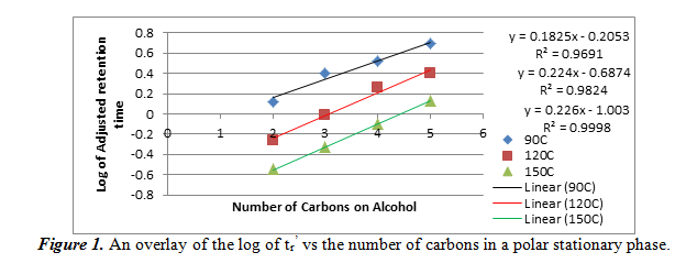
On this graph, the equations of the lines on the right correspond to the positions of the lines: the blue line, which is on top and is for the data at 90^oC, corresponds to the top equation and R² value, etc. As it can be seen, the relationship between the log of t_r^’ and the number of carbons is linear. Our R² values were all greater than 0.96, meaning that it was a very good linear fit. We can also note that the adjusted retention times decreased as temperature increased for the same alcohol. This data wil help us determine our unknown if we use this polar stationary phase.

Next, we create a plot of the log of t_r^’ vs the reciprocal of the column temperature for each alcohol. From this graph we can see the relationship of the temperature and the number of carbons on the alcohol on the adjusted retention time. The graphs are shown below in figure 2.

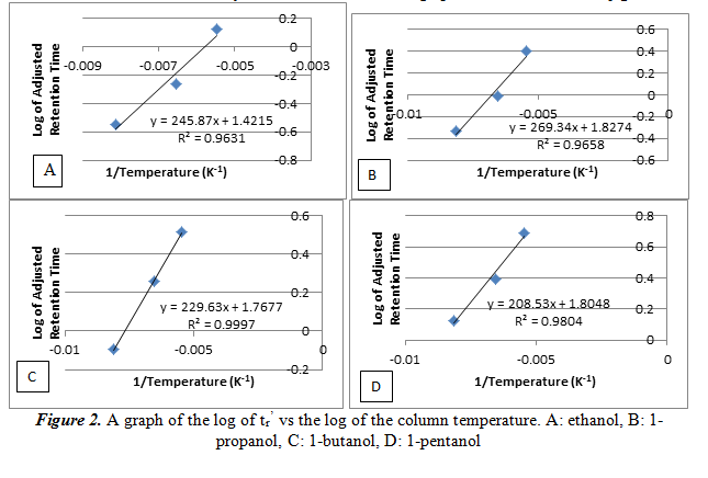
As it can be noted on the graphs, the log of t_r^’ increases linearly as the reciprocal of the temperature increases. This is another way of saying that the relationship between the log of t_r^’ and temperature is inversely proportional. The large R² values, each greater than 0.96, shows that the data has a good linear fit line. These data will also help determine our unknown.

2.2 – Non-Polar Stationary Phase

For this section, we repeat what we did for section 2.1, but used a non-polar stationary phase. The same temperatures were used, and we created a graph of the logarithm of the t_r^’ vs the number of carbons in the each of the four alcohols in figure 3.

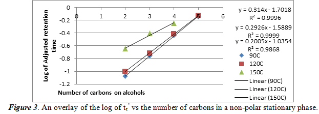
As one can see, in a non-polar stationary phase, the relationship of the log of t_r^’ is still a positive linear correlation. The high R² values show that these data have a good linear fit line. An important aspect to note is that the chromatogram taken at 150^oC only showed 3 peaks. This means that 150^oC, there is bad separation of the four alcohols. The best fit line equations are ordered where the top equation and R² value is for 90^oC and the bottom set is for 150^oC.

Next, we create another plot of the log of t_r^’ vs the reciprocal of the column temperature for each alcohol. From this graph we can see the relationship of the temperature and the number of carbons on the alcohol on the adjusted retention time. The graphs are shown below in figure 3.

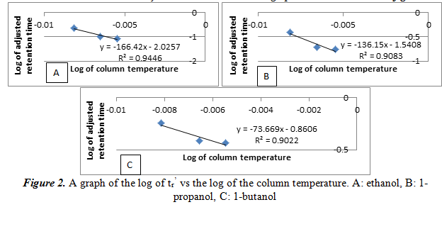
Similar to the results of 2.1, the log of t_r^’ increases linearly as the reciprocal of the temperature increases. Again, this is just another way of saying that the relationship between the log of t_r^’ and temperature is inversely proportional. The R² values here, however, are not large (only around 0.90). It is important to note that there is no graph for 1-pentanol, unlike section 2.1. This is because with only three peaks at 150^oC in the previous part, there is only two points for its graph, meaning it is impossible to create a linear best fit line. Also, this shows that there is poor separation with the non-polar stationary phase, and we will not use it for our experiment.

2.3&2.4 – Determination of the alcohols in the unknown

For this part, we performed a series of tests to figure out the optimal settings for separation of the unknown. We ran it at different temperatures and used the polar stationary phase. We found 100^oC to be the best condition for separation. In the following table 1, we will list the adjusted retention times of the six pure alcohols. We also put the retention times of the three determined alcohols in our unknown next to the closest value of the pure alcohols. We hypothesize that these three alcohols are in our unknown.

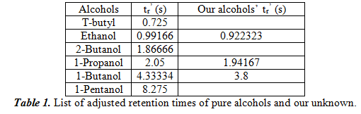
Additionally, we used a spike method where we added a large amount of the hypothesized alcohol to see if the peak area change (which is proportional to concentration) made an unambiguous change. The results confirmed our hypothesis that the three alcohols that are present in our unknown are ethanol, 1-propanol, and 1-butanol. Next, we chose one of the alcohols in our unknown, in our case 1-propanol, and did three more injections to see the uncertainty in calculating t_r^’. From the four trials we had, we got the result of 2.02485±0.03793s. With this value, we can calculate the uncertainty by dividing the standard deviation by the square root of the number of elements we used (which is 4^0.5=2). Therefore, the uncertainty is 0.01896s.

2.5 – Sensitivity Factor and Quantification

For this part, we will compare the peak area to the amount of alcohol that is present in the standards and our unknown. We do so by doing a total of four measurements of the three pure alcohols in our unknown and find the average. In the end, we get 0.05915±0.00805 for ethanol, 0.06025±0.00300 for propanol, and 0.06298±0.00376 for 1-butanol. These peak area values correspond to approximately 2µL of each of the pure alcohols. Therefore, the sensitivity factor is each of the peak areas divided by 2. This gives 0.02958µL^-1 for ethanol, 0.03013µL^-1 for propanol, and 0.03149µL^-1  for 1-butanol. To figure out the amount of each alcohol in our unknown mixture, we must figure out the average peak area from our trials (which are 0.0368±0.005 for ethanol, 0.0113±0.001 for propanol and 0.0102±0.001 for 1-butanol), then divide by the sensitivity factor of the pure alcohols. From this we get 1.24µL ethanol, 0.37µL propanol, and 0.32µL 1-butanol. In the following table 2, we can also get the volume percent, weight percent, and molar percent of the alcohols.

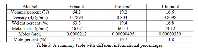
For the table, to calculate weight percent, equation 1 was used. For calculating moles, equation 2 was used. For mole percent, equation 3 was used. The total weight for the samples is 0.00154g.

1. Weight percent = V_alcohol * d / m_tot  * 100%
2. Moles = m_alcohol / m_molar
3. Mole percent = moles / moles_tot * 100%

Discussion and Conclusion

This experiment was done to study gas chromatography and attempt to successfully separate an unknown mixture of alcohol into its components. We then would quantify and identify the alcohols present. Through a series of experiments, we were able to identify the conditions that produced optimal separation. These conditions were at 100^oC and with the use of a polar stationary phase. With no overlapping peaks, this condition was used to study our unknown.

The original peak percentages for the three alcohols are 62.2% for ethanol, 18.7% for propanol, and 16.2% for 1-butanol. Comparing these values to the mole percent, it seems that ethanol’s mole percent is moderately greater than the original peak percentage, while propanol and 1-butanol’s mole percent was slightly lower than the original peak percentage.

Using  figure 1, we can compare the log of adjusted retention times of the alcohol to the number of carbons. For ethanol, propanol, and 1-butanol, respectively, the log values come out to be -0.0351170, 0.288175, and 0.579784. These values fit into the areas between the 90^oC and the 120^oC best fit lines, meaning that it confirms the identities of the unknowns. Also from section 2.1 and 2.2, we can see the effect of temperature and number of carbons atoms on the adjusted retention time. As temperature increases in a polar stationary phase, the adjusted retention time decreased for the same number of carbons. This is probably because higher temperatures vaporized the alcohols faster so it can travel faster. Then, when the number of carbons increased, so did the adjusted retention time. This is probably because the boiling points increase with number of carbons, which means that vaporization took longer. For a non-polar stationary phase, the conditions were the opposite. Each of the two relations found in polar stationary phases are inverted for a non-polar stationary phase.

There are several errors present in this lab. One is that sometimes the gas chromatograph is inaccurate with the baseline placement when calculating peak areas and peaks when recording data. A second error is that the amount of alcohol injected into the gas chromatograph may not have been 2µL, as the syringe may not be accurate. Also, since the volume is on such a small scale, small deviations may cause a large amount of error. This may not only happen during the experiments with the unknown, but also with the standards and manifest in large ways.