Green’s Theorem and Vector Fields
Introduction:
In this lab, we examined fundamental properties of vector functions and vector fields in two different problems using concepts we learned in chapters 13 and 14. In the first problem, we explored gradient fields, flux, flow, divergence, curl of vector fields, and investigated Green’s theorem to determine how flux and divergence are connected, as well as flow and curl. In the second problem we looked at the first and second moments of a charged surface.
Results:
In the first part of the lab, we constructed the function f in polar coordinates and analyzed the gradient field. Our given surface was z=f(r, theta) defined on the domain r is including and between 0 and 1, and theta is including and between 0 and Pi.
Equation 1:
Provided with the given gradient field

we needed to find f(r ,theta). Since nr^(n-1)*sin(nq) is the derivative of F(r,q) with respect to r, and nr^(n-1)*cos(nq) is the derivative of F(r,q) with respect to q, we knew that to find f(r,q) we only needed to integrate either F with respect of r or F with respect to q since both would yield the same function. We determined f(r,q) to be r^(n*sin(nq)).
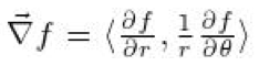
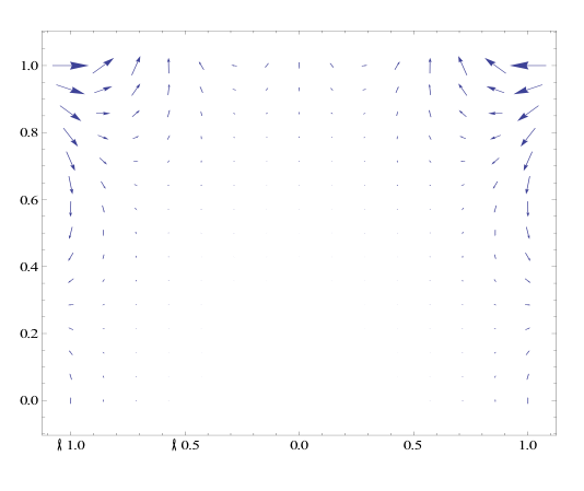
Next, we plotted f(r ,theta) and its gradient field for n={ 1,2,4,7} using the Mathematic function ManipulateVectorPlot[ ]. In order to do this, we had to convert the gradient field from polar to Cartesian coordinates by defining functions r(x,y) and theta(x,y).The plots show the gradient fields which essentially represent the slope of the contour at a give point. So at the beginning the surface is flat and our plot is all arrows strait up. Then once we change n the gradient field changes to go along with the slope of the surface so the gradient plots will now bend all around as you will see in our plots. We will show plots when n=1, 2, 4,7.
Gradient Field when n=1
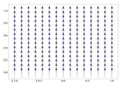
Gradient Field when n=2
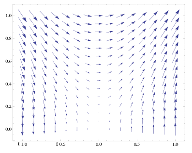
Gradient Field when n=4
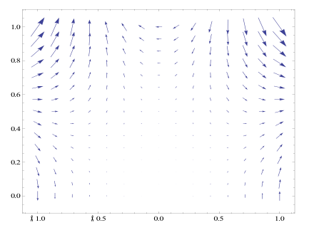
Gradient Field When n=7
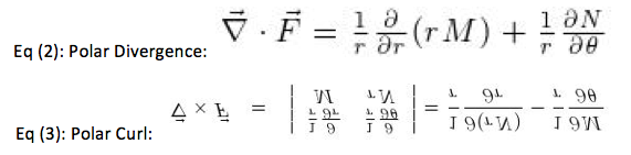
We were able to find the Polar Divergence, and the Polar Curl of the given function F(r,theta) using equations 2 and 3, respectively. We found the polar curl and divergence to both be zero.

We found that F is conservative and exact. The gradient field of a continuously differential function f is always conservative because it is path independent. The line integral of a continuous gradient field along a path only depends on the endpoints of the path. F is also an exact differential form. To prove that F was conservative, we made sure ∂ P/∂ y= ∂ N/∂ z, ∂ M/=∂ P/∂ and ∂ N/∂ x=∂ M/∂ y, and indeed they were. A differential form is exact on a domain in space if M dx + N dy + P dz= df. The test for F’s being conservative is actually the same as the test for the form’s being exact, thus, F is conservative and exact.
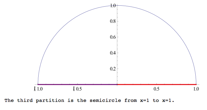
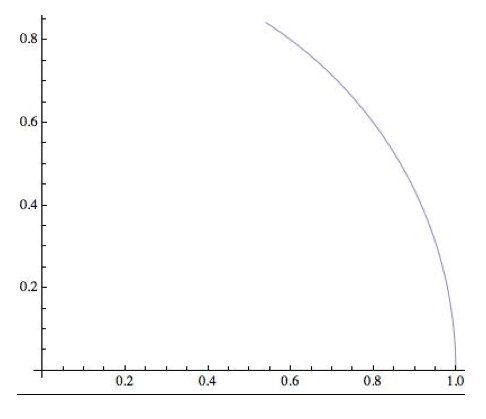
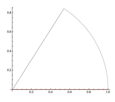
Next, we confirmed that the flux of F is zero across the domain. To do this we considered the boundary of the domain to be defined by a closed contour defined by the x-axis, x is including and between -1 and 1, and the upper half of the unit circle, and partitioned this contour into three parts using polar coordinates. The first contour was defined by r=1 , and theta is between and including 0 and Pi. The second contour is given by theta =0, and r is between and including 0 and 1, and the third contour is given by theta is Pi, and r is between and including 0 and 1. We plotted each of the sections separately to see that the flux of F was zero in each plot. Next, we computed the flux of F across each of these contours by integrating counterclockwise, and concluded that the flux was zero.
First partition:
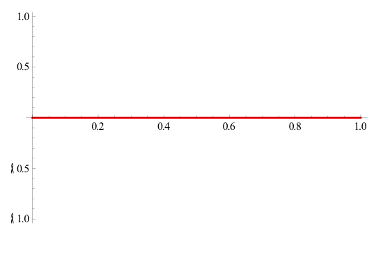
Second Partition:
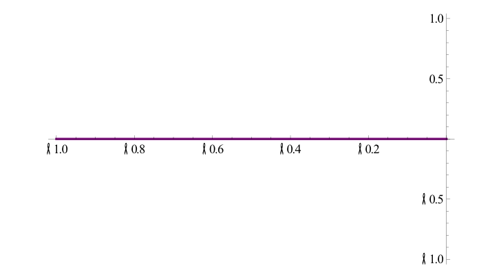
Complete Curve:
The flux divergence form of Green’s theorem is the integral of F dot n ds over the closed curve c is equal to the integral of M dy – N dx over the closed curve x, which is also equal to the double integral of (∂M/∂x +∂N/∂y) dx dy over the region R enclosed by C .This means that the outward flux of a vector field, F=M i + N dx, across a closed curve in a plan is equal to the double integral of divergence of the field over the enclosed region by the curve. We evaluated the double integral in Green’s theorem over the domain in question 4 and found that it is equal to our answer to question 4, both being zero.
The circulation-curl form of Green’s theorem is the integral of F dot T ds over the closed curve c is equal to the integral of M dx + N dy over the closed curve c is equal to the double integral of (∂N/∂x – ∂M/∂y) dxdy over the region R enclosed by C. This means that counterclockwise circulation of a field, F=M I + N j around a closed curve C in a plane is equal to the double integral of curl F over the region R enclosed by C. We found that the flow of F around the contour described in question 4 was 0. To do this we parameterized M and N using x= cos(t) and y= sin(t), respectively, and integrated Mdx +Ndy from zero to pi. The flow of F around C is the same integral of the curl of F over the domain. Curl is the circulation flow density; therefore integrating the flow around the region is the same as finding the curl over the domain.
Next we wanted to prove that the flow and flux of F are zero around any closed contour in the domain. We first found the flow and flux of F around a wedge in the domain of F that goes from r= r0 to r=r1, and theta = theta0 to theta = theta1, 0 ≤ro≤r1≤1 and 0≤ theta0 ≤ theta1≤1. We partitioned the closed contour into four pieces. These four pieces create curve long the x axis to r=1 then creates an arc with r being constant at 1 and theta goes from 0 to 1, then it goes strait back to the origin.
Contour 1
Contour 2
Contour 3
Complete Curve
We computed the flux and flow through every partition of the contour and added them to find that both the flux and flow are zero. We also found that F is conservative because ∂ P/∂ y= ∂ N/∂ z, ∂ M/=∂ P/∂ and ∂ N/∂ x=∂ M/∂ y. Because F is conservative, the flux and the flow around any closed curve in the domain is zero.
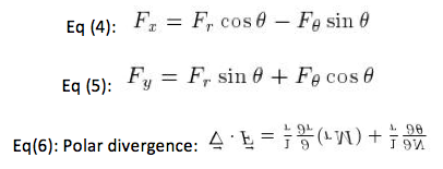
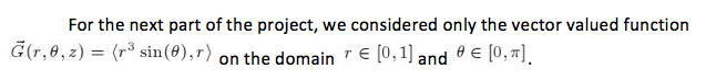
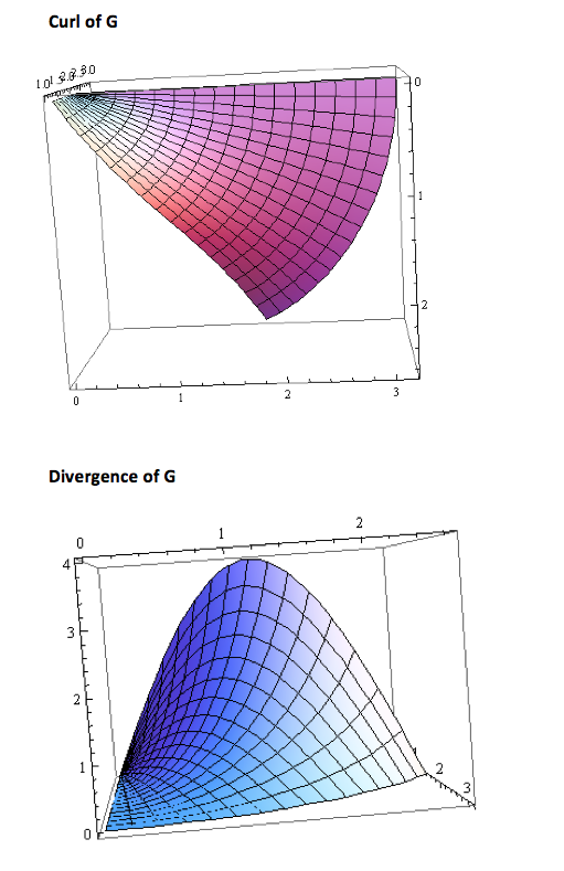
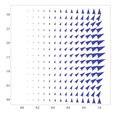
We first converted G(r, theta , z) from polar to Cartesian coordinates in order to find Gx and Gy using equations 4 and 5 (substituting G for F). From Gx and Gy, we found the vector G and plotted the vector field G. By looking at the graph, I could see that x went from -1 to 1, thus in polar coordinates theta went from 0 to pi, which is the region for integration that we used to find the flow of G around the perimeter of the domain. From the graph we also determined that x=cos(t) and y=sin(t). Therefore dx=-sin(t) and dy=cos(t) . To find the flow of G, we integrated M dx + N dy from 0 to pi in which we parameterized r and theta and substituted from M and N respectively. From this calculation, we found that the flow of G around the perimeter of the domain is zero. G is not conservative because G doesn’t meet the conditions of ∂ P/∂ y= ∂ N/∂ z, ∂ M/=∂ P/∂ and ∂ N/∂ x=∂ M/∂ y. G cannot be written as a potential because G is not conservative. We also used the given function G to find the divergence of G from the domain using Eq (6). We found the divergence of G to be 4*r^2*sin(2q). This is the same value as the flux through the boundary of the domain.
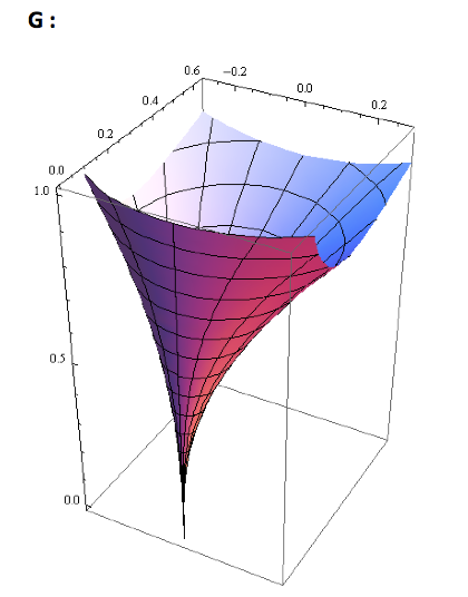
Vector Field of G:
Conclusion
In this project we used concepts from chapters 13 and 14 to explore vector-valued functions and their vector fields. We exploring vector fields, and were able to obtain a much better understanding of fields of force that occur in the natural world. By representing a force as a vector field it allowed us to comprehend how a force acts over a region, rather than just at a point. Throughout the lab we came to realize that there are many types types of vector fields, called conservative fields, which have distinctive and important properties. Some of these properties are: the idea that the work of an object is path independent, the flow around a closed loop is always zero, and the fact that the flux in the region is also zero. All of these properties are important because once a field is determined to be conservative we automatically have information about the work, flow and flux in the region.
