Green’s Theorem and Vector Fields
Introduction
For this lab I observed the properties of Vector fields and functions. For the first problem I examined gradients, divergence and curl operators to further understand Green’s Theorem. This helped identify the links between divergence and flux, as well as curl and flow. For the second portion of the lab I examined the properties of the first and second moment on a charged surface.
Problem I
For the first portion of the this lab I used the given information to constructed a function that defined the surface z=f(r,q) over a domain such that, r is greater than or equal to zero and less than or equal to 1, and that q is greater than or equal to 0 and less than or equal to Pi.
With the provided gradient field:

In knowing that the gradient of function is the partial derivate of a function with respect to a certain variable, I deduced that by integrating either partial derivative with respect to its differentiated variable, the original function, F(r,q) could be obtained. By following the procedure is found that F(r,q)= r^(n*sin(nq)).
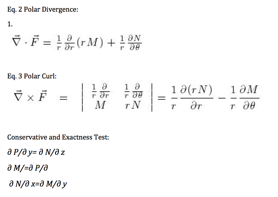
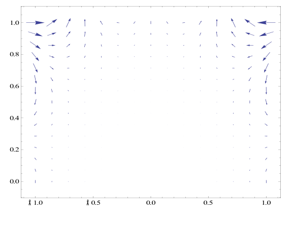
From here I plotted F(r,q) and its gradient field for n={1,2,4,7}. For this to be done I first defined the radius and theta variables in terms of x and y, in Mathematica By doing this I converted the gradient field equations into Cartesian coordinates. After this was done I used the VectorPlot[] in Mathematica to give a visual representation of the field. Below shows the plots over the various values of n.
Grad. Field n=1
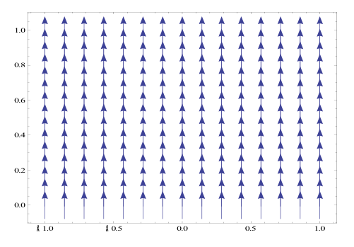
Grad. Field n=2
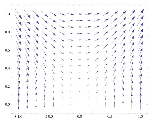
Grad. Field n=4
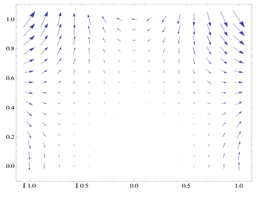
Grad. Field n=7
After I plotted the above transformations I found the Polar Curl and Divergence. To do this is used equations two and three.
In computing these equations I found that the both the Polar divergence and curl were equal to zero.
Using techniques that I learned in Chapters thirteen and fourteen, I found the function to be both conservative and exact. I found this by realizing that the function is continuously differentiable it must conservative because it is independent of its path meaning it is also exact. To check this mathematically rather than conceptually I used the conservative test, which is also a test for exactness.
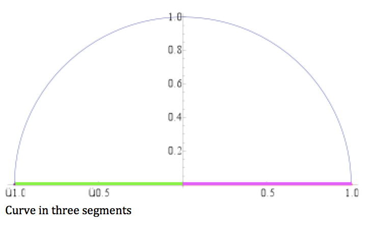
After conducting these test’s I verified that the flux across the boundary of the domain equals zero. To prove this I defined the domain to be a half circle of radius 1 units; this circle is closed, such that it consists of three different segments (below). The first segment extends from r=0 to r=1 along the x-axis, the second is a half circle of radius one from theta equals zero to pi, and the third is a line segment from r=0 to r=-1. With a counter-clockwise path I integrated each piece separately and worked out that the flux across the boundary did in fact equal zero.
The flux-divergence form of Green’s theorem is the integration of F dotted with N over the closed curve C. This formula can also be written as the double integral of (∂M/∂x +∂N/∂y) dx dy). This formula can be interpreted such that the outward flux across the enclosed region of the curve is equal to the divergence across that same curve.
Appendix