Mathematica – Calculus Lab
Introduction
In this lab we will use Mathematica to perform many mathematical operations. We will further expand our knowledge of vectors by using the Mathematica program. This program will allow us to demonstrate the properties of dot products versus cross products. The purpose of the lab allows for us to become familiar with the numerous commands of Mathematica. These commands include NSolve[], Integrate[], Simplify[], and many more. We will also be able to use and apply Mathematica’s graphing capabilities. We will learn to graph many different types of surfaces, as well as solve complicated real life problems. Using Mathematica we can evaluate infinite series and to evaluate infinite sums. By applying our knowledge of mathematics, this lab should assist us in solving real world problems in a simpler manner.
Body:
Problem 1.1
The dot product of two vectors results in a scalar. The dot product is determined by multiplying the x, y, and z-components of one vector by the x, y, and z-components of the other vector, and then adding up the three numbers together. The dot product of V2 and V3 resulted in 6.
V2 * V3
Multiply the x, y, and z components: (V2x*V3x= 3, V2y*V3y=2, V2z*V3z=1)
Add the products: 3+2+1=6
The same concept is used for finding the dot product of V3 and V4, which resulted to be 3. These resulting scalar numbers represent one vector’s magnitude times the other vector’s projection onto the first vector. For example the dot product of A and B is the magnitude of A times the projection of B onto A. Finding the dot product of the same two vectors (meaning they both have the same magnitude and same direction) is found the exact same way. Therefore, the dot product of V3 and V3 is 11. This value is the magnitude of V3 times the projection of V3 onto itself.
The magnitude of V2+V3 is <4,3,2>.
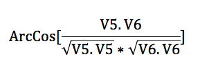
An additional definition of the dot product is the magnitude of one vector times the magnitude of another vector times cosine of the angle between the two vectors. Therefore, if the angle between the two vectors is zero, meaning that the two vectors are in the same direction, then the cosine of zero is equal to one. Cosine of zero is the max cosine will be. Now if the goal is to determine the angle between two vectors just find the dot product of those vectors, divide by both their magnitudes, and then take the inverse cosine of the result.
The V5 vector only has an x-coordinate. The V6 vector has both an x- and y- coordinate but not a z-coordinate. If we were to guess the angle between vector V5 and V6 we would assume it to be 45 degrees (pi/4 in radians). Think of the “triangle” the two vectors make. V5 will point along the x-axis one unit. V6 will point at 45 degree angle in the first quadrant because it goes along the x-axis one unit and up the y-axis one unit. Therefore this is a 45-45-90 right triangle and the angle between V5 and V6 should be 45 degrees.
Problem 1.2
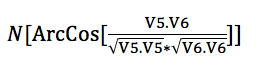
In Mathematica there are two functions called NSolve[] and Solve[]. The NSolve[] function gives a list of the numerical approximations of the roots of the function enclosed by the brackets. The Solve[] function solves the function enclosed in the brackets. The Solve[] function is extremely helpful because it gives an exact result. The ArcCos[] function finds an angle and expresses the results in the radians.
Problem 1.3
Using the Solve[] function we found the angle between V2 and V3 to be pi/4 radians like we had assumed above.
Problem 1.4
There are two additional functions called Integrate[] and NIntegrate[]. The NIntegrate[] gives a numerical approximation just like the NSolve[] stated earlier. Also, the Integrate[] function gives an exact result. We used both the functions to find the integral of x^2*Sin[x^3] and Exp[-x^2] over the interval from 0 to 1. The Integrate[] gives a better result because it is more precise, versus NIntegrate[] gave an approximation of the integral.
Problem 1.5
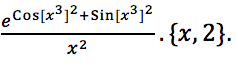
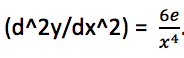
We calculated the second derivative of y(x)=exp[cos^3]^2+sin[x^3]^2]/x^2 by using the D[] command. We plugged in the y(x) function and specified to find the second derivative as follows D[f[x],{x,2}]. The second derivative was found to be
Using the Simplify[] command the result was
Problem 1.6
The cross product of V1 x V2 resulted in .The cross product of two vectors results in another vector unlike the dot product. The resulting vector is normal to both the vectors originally crossed. For example, A x B will result in a vector that is normal or perpendicular to vector A and vector B. Therefore, our resulting vector found for V1 x V2 is another vector that is normal to V1 and V2.
Problem 1.7
We can also cross a cross product with another vector such as (V6 x V7) x V8.
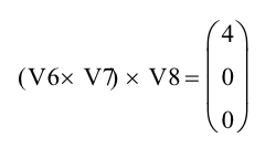
The cross product of V6 x (V7 x V8) is below.
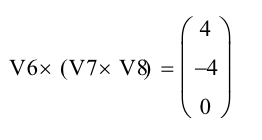
This result is different than the result found from (V6 x V7) x V8. If we dot product a cross product it is ok to rearrange the order of where the scalar is; A * (B x C) = (A x B) * C. The reason for this is A x B = -(B x A). This shows that the direction of a cross product varies with the arrangement of the vectors. The cross product is not associative. Dot products however are commutative.
Problem 1.8
Below are the cross products of V1 x V10 and the cross product of V10 X V1.
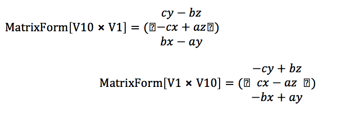
These products are in opposite direction of one another.
Problem 1.9
Problem 2.1
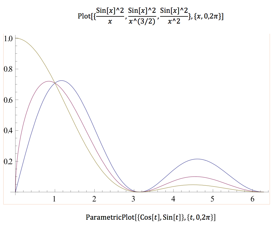
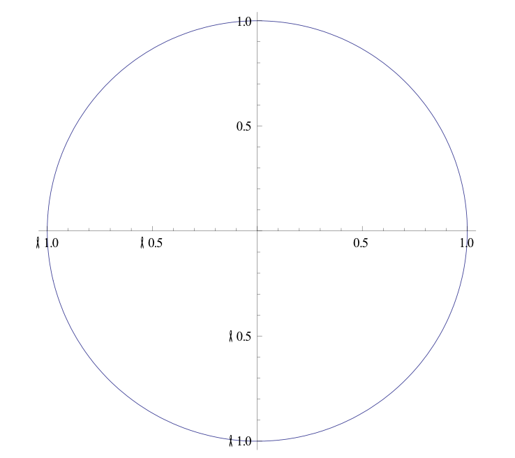
We plotted the graphs of sin[x]^2/x, sin[x]^2/x^(3/2), and sin[x]2/x2. Additionally, the circle x^2+y^2=1 is plotted as well below.
Problem 2.2
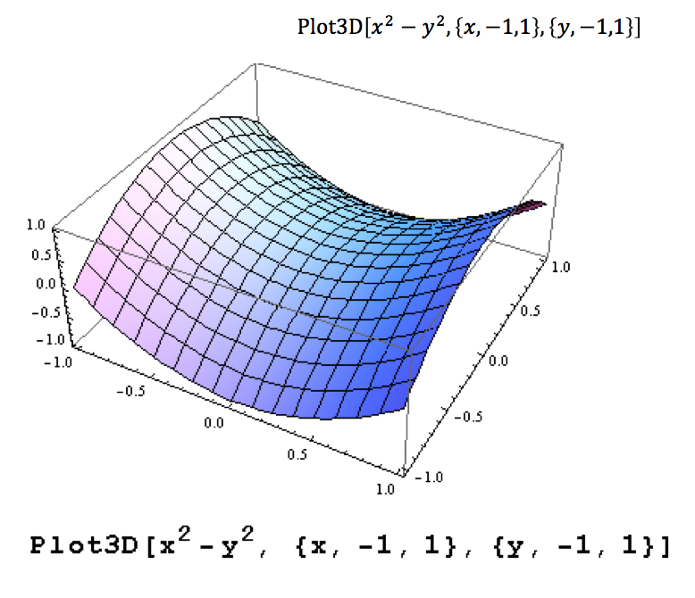
Now we used the Plot3D[] command which forms a 3-dimensional plot of the functions. For example we plotted x^2-y^2 in 3-D as below.
Problem 2.3
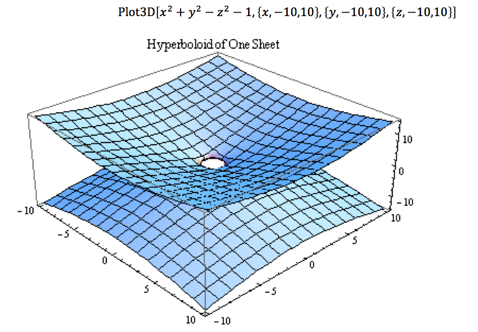
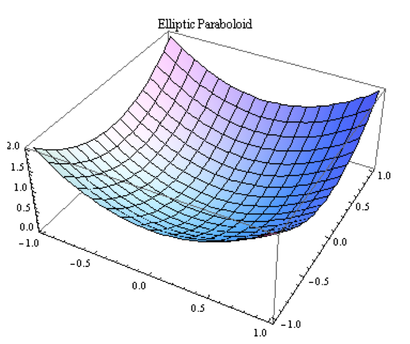
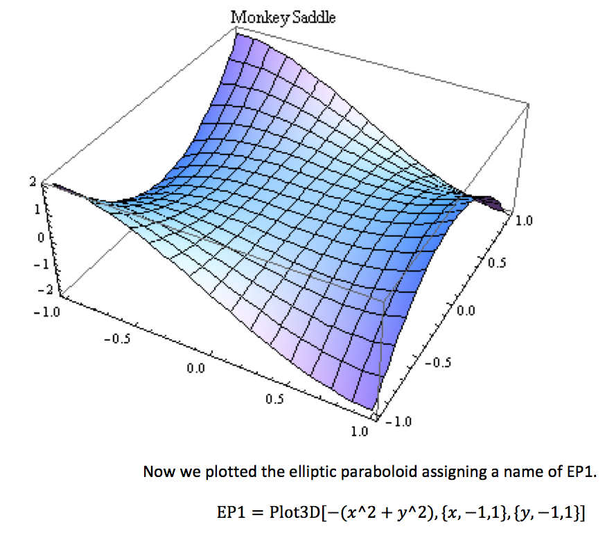
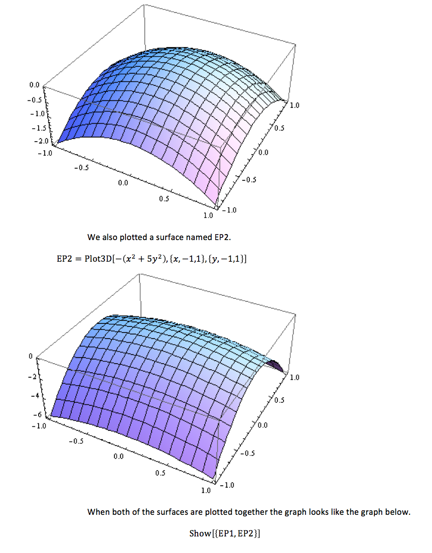
The following graphs represent quadratic surfaces. The first graph is a hyperboloid of one sheet which has the general equation x^2/a^2 + y^2/b^2 –z^2/c^2 = 1. The second graph is an elliptic paraboloid. Elliptic paraboloid’s have the general equation of x^2/a^2 + y^2/b^2 = z/c. The third graph is called a “monkey saddle”. This surface has the equation of : x3-3*x*y2. This surface is not considered a quadratic surface because there is no x^2 term. Quadratic surfaces have the general equation of Ax^2 + By^2 + Cz^2 + Dxy + Eyz +Fxz + Gx +Hy + Jz +K = 0. Remember that the capital letters are just constants.
Problem 2.4
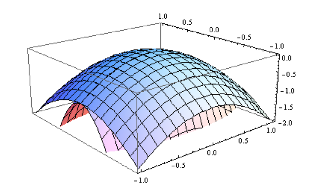
This plot is to show how the changes in parameters cause changes in the figures. We combined a series of plots to be in one.
Problem 2.5
(For this problem please refer to the Appendix for coding located at the end of the lab.)
The purpose of this problem is to make 1-inch drill bits. There are four other options of drill bit sizes: ½-inch, 2-inch, 3-inch, 4-inch.
Problem 3.1
We evaluated the series below and found the results. The result of Eqn. 3.3 is pi^2/6. The first series, Eqn. 3.2, does not converge to a value because it is divergent. These are convergent infinite series. This means that they converge to some real numerical value. Convergent infinite series is basically a sequence of partial sums given a sequence of numbers. Let’s say the sequence of numbers is
is the infinite series. If this series add up and converge then there is a convergent infinite series. If they do not the series is divergent.
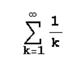
Eqn. 3.2
The series diverges because the harmonic series in 1/n diverges.
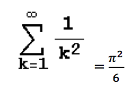
Eqn. 3.3
The series converges using the P-Series Test because P is greater than 1.
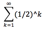
The infinite series below converges to one.
Problem 3.2
The length of the finite vector from equation 3.12 which is defined below is just the square root of A^2. That is the equation of the magnitude of vectors. .
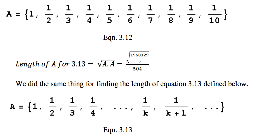
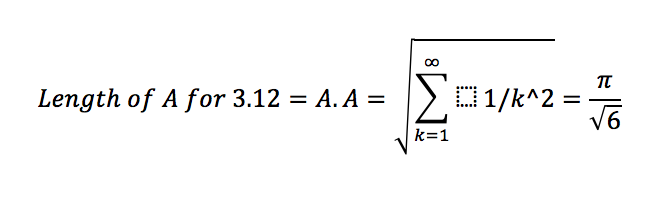
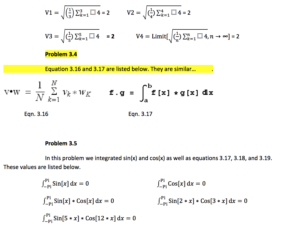
Problem 3.3
The length of the vector V1 = {2,2,2} is 2. The length of the vector V2 = {2,2,2,2} is 2. The length of the vector V3 = {2,2,2,2,2} is 2. The length of the infinite vector V4 = {2,2,…} is 2. For the infinite vector we had to use the Limit[] command.
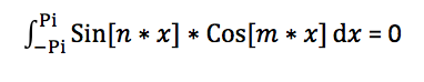
If we consider the integral to be like a dot product we can conclude that the sine and cosine functions are perpendicular. This concludes that the dot product of perpendicular vectors is zero. We knew this fact from before. Adding constants of m and n does not alter the result at all because the vectors are still perpendicular to each other.
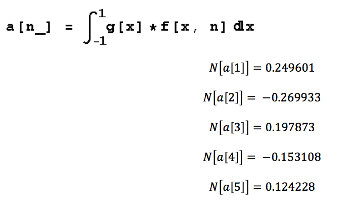
Problem 3.6
In this problem we evaluated a[n]; n is equal to one to 5. The equation for a[n] is defined below. We used the N[] function to find the values of a[n] from n=1 to n=5. The values for each corresponding n are stated below.
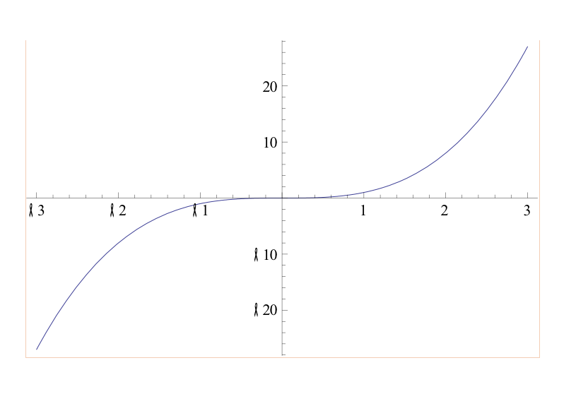
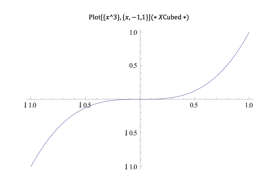
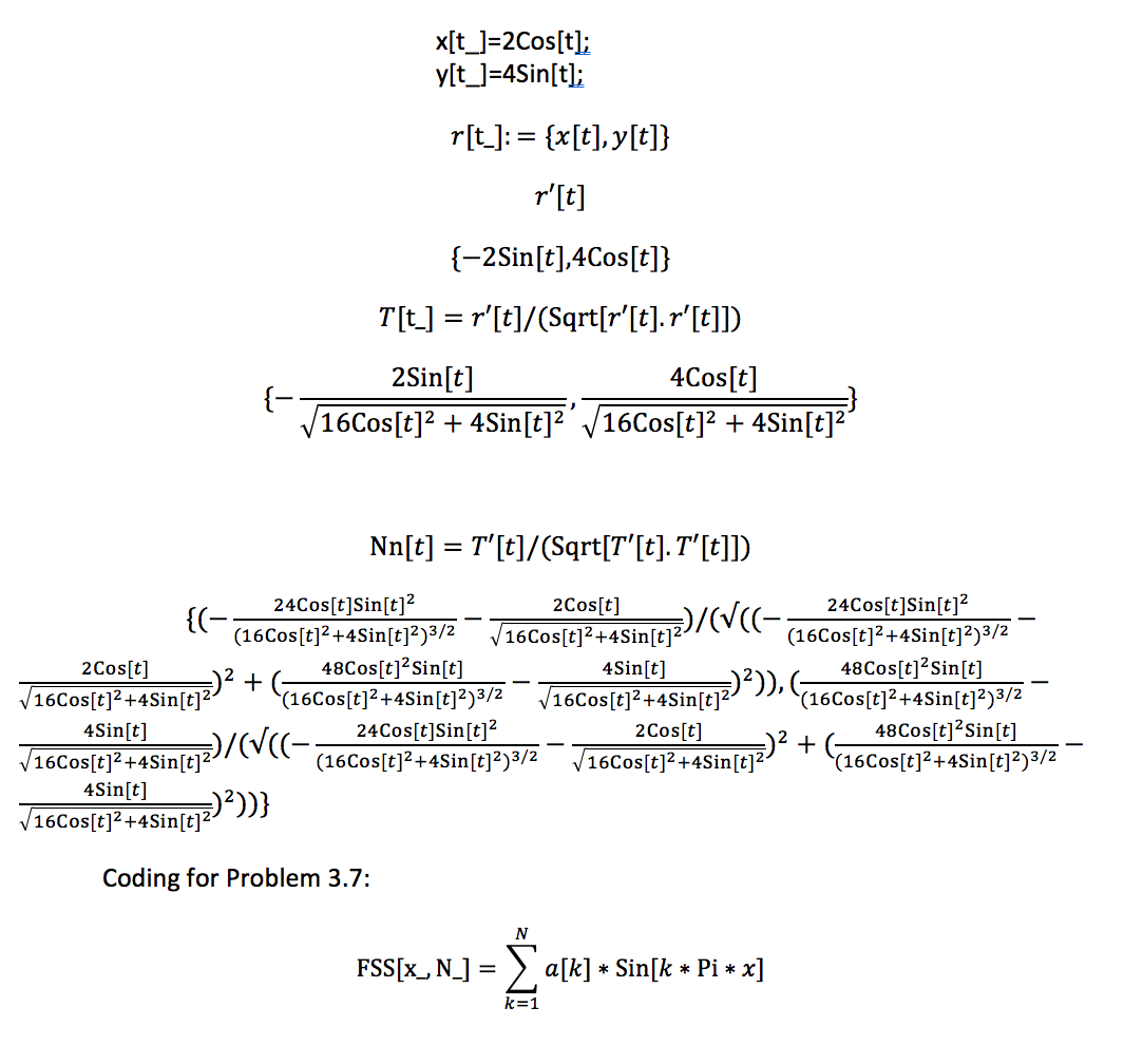
Problem 3.7
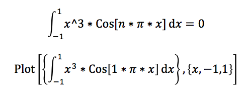
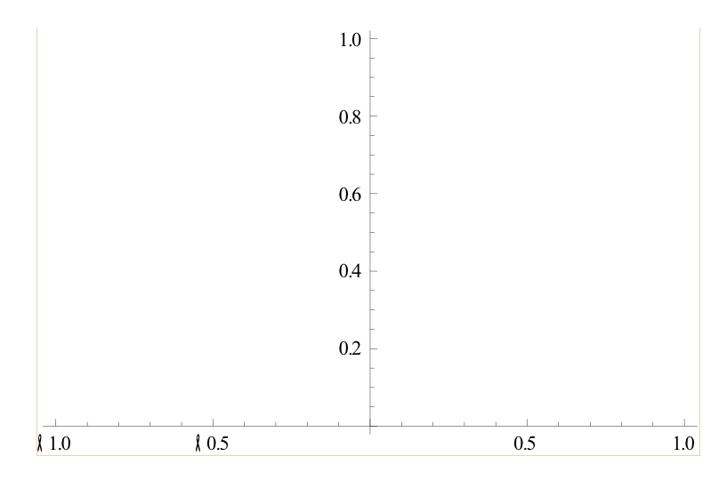
Equation 3.26 and its result is stated below. Because the graphs of the functions are symmetrical the net area under their curves is going to equal zero. We plotted the integrand, equation 3.26, for different values of n. The graph came up as the one below the equation. The graph looks like nothing is plotted. This is because the integrand of this symmetrical function from (-1,1) is zero. Therefore, no matter the value of n, the integrand will equal zero.
Problem 3.8
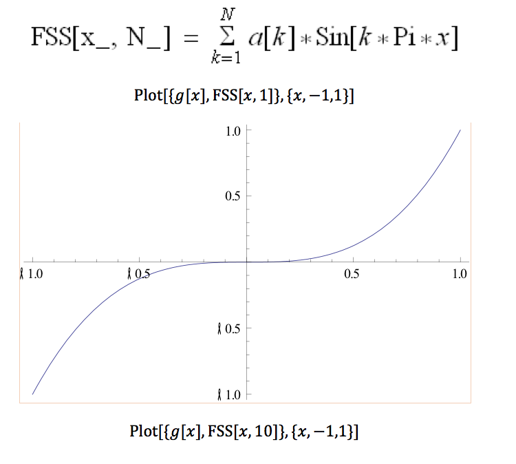
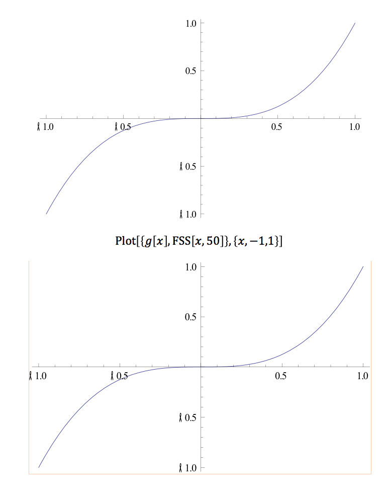
In this problem we graphed FSS[x,n] from (-1,1) for n=1, n=10, and n=50. The three graphs are in order below. Each of the graphs look exactly alike.
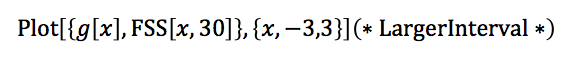
Problem 3.9
The graph of FSS[x,30] on (-1,1) is going to look exactly like the graphs above. This shows that the Fourier Sine Series of a function is independent of the value of n. The interval of (-3,-1) looks exactly like the interval from (-1, -.05). The graph of this is below.
Conclusion
Appendix
Coding for Problem 2.5:
PDF version of this post is available here: Lab #1 Write Up
