Calibration of Micropipette and Peristaltic Pump
Calibration of Micropipette and Peristaltic Pump
By: Andrew Tam
Part 1 – Calibration of Micropipette
Results and Discussion:
We took a micropipette and pipetted out water of volumes 100, 250, 500, 750, and 1000 uL at specific temperatures (for our experiment, our temperature was 22.9oC) and recorded the mass of the water that was ejected from the micropipette in five trials for each setting. We then convert this value back into uL in order to compare the amount delivered at each separate setting using the following equation (1).
(1) . Volume delivered(uL) = mass recorded(g) / density (g/mL) * 1000 (uL/mL)
We were able to do so by plotting the average volume delivered versus the dial setting. This procedure generated a calibration curve, shown below in Figure 1.
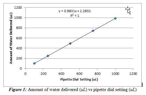
From Figure 1, we observed that the pipette behaved as expected; the amount of water delivered increased with the pipette dial setting. It can also be said that this relationship is practically linear due to the slope being relatively close to one (slope = 0.9831±0.0003). The intercept is then noted to be 2.283±0.175 uL. This value shows that even at a pipette setting of 0 uL, the pipette will still deliver around 2.283 uL. The line is also a very good fit (R2= 1) for the data set. It should be noted that the error bars are present, but they are on a scale too small to be observed on this graph, meaning there is a lot of precision in my pipette.
We can then use the equation from this linear regression line to identify how much water should be delivered by the pipette based on the dial setting. Ideally, we would want the slope to be one and have an intercept of zero because the amount of water delivered must be accurate and have a linear relationship with the pipette dial setting. The standard deviations of the slope and the intercept are small, relative to the resulting value, so the standard deviations are not very significant.
Next, we have to evaluate if the means of our values at 250 and 500 uL are statistically different than the class mean at a 95% confidence level.
One method is where we consider the class average to be the true value (µ) and our mean (x̄) is an experimental average from a limited number of measurements (n=5). To do this, we must use the standard deviation of our data set and find the t-value using this equation (2).
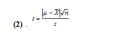
Using our mean and standard deviations of 248.0±0.7 uL and 493.7±1.8 uL, for the 250 and 500 uL dial setting, respectively, and the class means of 259.5 and 506.2 uL, we get t-values of 36.74 and 15.53. With 5 degrees of freedom, these t values are larger than 2.57, which means that our means are statistically different than the class mean value at a 95% confidence level.
The second method uses a pooled t test by not considering the class average to be the true value. We then must calculate a pooled standard deviation from the following equation (3).
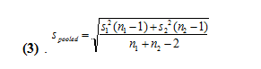
We get values of 37.3 and 35.7 for the pooled standard deviations for 250 and 500 uL, respectively. We then use the following equation (4) to find the pooled t-value.
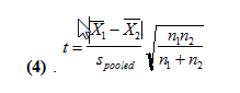
With this, we find the t values to be 0.678 and 0.770. At n1+n2-2 degrees of freedom, t can be at most 1.66 for the two means to not be statistically different. Since our two t values are less than 1.66, this means that with the second method, our mean amount of water delivered are not statistically different at a 95% confidence level.
Conclusions:
This part of the experiment was to determine of the pipette we received was correctly calibrated with respect to the other pipettes of the laboratory class. This was done by creating a calibration plot and calculating the statistical difference between our means of water delivered based on a certain pipette dial setting. The results show that there is a linear 1-to-1 correlation of the pipette dial setting and the amount it delivers. Also, the pipette was accurately calibrated to the amount it reads on the dial.
There seems to be a huge difference when we use each of the two methods of determining the statistical difference between the means. This could be attributed to the fact that the first method suggests that the class mean is the true value, which is not true, as the true value is never known for sure. Also, the second method more correctly calculates the difference by comparing the two means in a pooled technique, without labelling one of the values to be the true value.
There are a few sources of error for this experiment. Some examples include the fluctuation of the mass balance when recording values for the data table. There was also a very significant error in the class data set. The entries that correspond to 4A with pipette number 138 delivered around 447 uL at the dial setting of 250 and around 690 uL for 500. This skewed the class average to be a value higher than what it should be. Also, the water on the balance can evaporate as data is being recorded and successive trials are being performed. Also, we recorded the temperature of the water that was being pipette to have an accurate density conversion, but the temperature of the water might have changed during the course of the experiment, which would have affected the data we received.
Part B – Calibration of Peristaltic Pump
Results and Discussion:
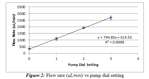
We took a peristaltic pump and recorded the flow rate of the water it delivers at one minute increments. We used 4 different dial positions to determine the relationship of the flow rate and the dial setting. These dial settings were at the 12, 3, 6, and 9 o’clock position, but for simplicity’s sake, we denoted them as 0, 1, 2, and 3, respectively on our graph and data. The temperature is 22.4oC. Equation (1) was used again to convert mass of water on the mass balance to a volume reading to more accurately perform this experiment. The time was measured by a stopwatch in minutes. The flow rate (uL/min) versus dial setting was used to generate a calibration curve that is shown below in Figure 2.
With this, we find the t values to be 0.678 and 0.770. At n1+n2-2 degrees of freedom, t can be at most 1.66 for the two means to not be statistically different. Since our two t values are less than 1.66, this means that with the second method, our mean amount of water delivered are not statistically different at a 95% confidence level.
Conclusions:
This part of the experiment was to determine of the pipette we received was correctly calibrated with respect to the other pipettes of the laboratory class. This was done by creating a calibration plot and calculating the statistical difference between our means of water delivered based on a certain pipette dial setting. The results show that there is a linear 1-to-1 correlation of the pipette dial setting and the amount it delivers. Also, the pipette was accurately calibrated to the amount it reads on the dial.
There seems to be a huge difference when we use each of the two methods of determining the statistical difference between the means. This could be attributed to the fact that the first method suggests that the class mean is the true value, which is not true, as the true value is never known for sure. Also, the second method more correctly calculates the difference by comparing the two means in a pooled technique, without labelling one of the values to be the true value.
There are a few sources of error for this experiment. Some examples include the fluctuation of the mass balance when recording values for the data table. There was also a very significant error in the class data set. The entries that correspond to 4A with pipette number 138 delivered around 447 uL at the dial setting of 250 and around 690 uL for 500. This skewed the class average to be a value higher than what it should be. Also, the water on the balance can evaporate as data is being recorded and successive trials are being performed. Also, we recorded the temperature of the water that was being pipette to have an accurate density conversion, but the temperature of the water might have changed during the course of the experiment, which would have affected the data we received.
Part B – Calibration of Peristaltic Pump
Results and Discussion:
We took a peristaltic pump and recorded the flow rate of the water it delivers at one minute increments. We used 4 different dial positions to determine the relationship of the flow rate and the dial setting. These dial settings were at the 12, 3, 6, and 9 o’clock position, but for simplicity’s sake, we denoted them as 0, 1, 2, and 3, respectively on our graph and data. The temperature is 22.4oC. Equation (1) was used again to convert mass of water on the mass balance to a volume reading to more accurately perform this experiment. The time was measured by a stopwatch in minutes. The flow rate (uL/min) versus dial setting was used to generate a calibration curve that is shown below in Figure 2.
