Heat Transfer – Pool Boiling in a Saturated Liquid
Heat Transfer – Pool Boiling in a Saturated Liquid
By: Josh Lashbrook
Abstract
Experiment No. 5, Pool Boiling in a Saturate Liquid, was conducted in order to verify the boiling curve for nitrogen at 1atm, as well as walk through the steps of its original creation. The lab was done using liquid nitrogen and a two submerged copper spheres of different size. Nitrogen was used because of its extremely low boiling point. If water would have been used, time would have been wasted heating the copper spheres well above 100°C. However as it was, the balls were at an appropriate temperature at room level to begin experimentation. Temperature measurements were taken on both surface and core temperature of the spheres.
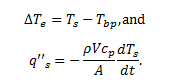
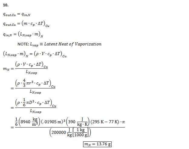
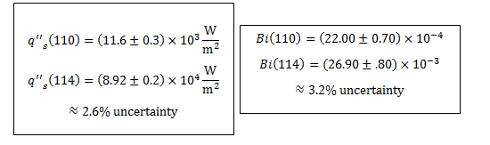
While data collection was done on both spheres, further data analysis only performed on the smaller sphere due to its lower Biot number and thus greater conformance to the lumped capacitance method requirements. The following equations were used in order to plot the boiling curve, the relationship between difference in sphere temperature and boiling point of nitrogen, and the contact heat flux between the sphere and nitrogen:
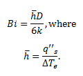
The Biot number was also found to verify that the lumped capacitance method is valid throughout the experiment using the following equation:
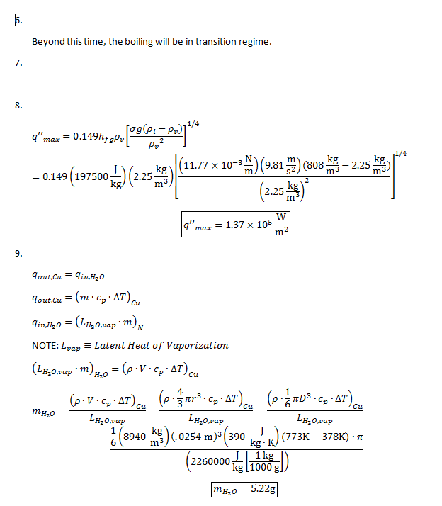
A theoretical q’’s,max and q’’s,min were found in order to compare our results with accepted values. Lastly, uncertainty calculations were performed to account for possible error.
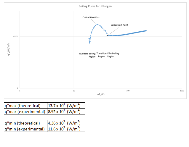
The produced boiling curve showed the main components of a boiling curve successfully. There were clear nucleate, transition, and film regions as well as an easily identifiable point of critical heat flux and a Leidenfrost point. We also were able to successfully prove that the lumped capacitance was valid all the way through the experiment. Based off calculated uncertainty, our heat flux uncertainty is 2.6%, and Biot number uncertainty is 3.2% uncertainty.
Theory
Outline
- Pour liquid nitrogen from storage container into test bottle.
- Prepare data collection by connecting the copper sphere thermocouples to the computer and initiate the DAQView data acquisition program.
- Submerge the sphere in the nitrogen while simultaneously triggering data acquisition on DAQView.
- Monitor sphere temperature until temperature levels off close to 77K, the boiling point of nitrogen.
- Stop data acquisition. Data will automatically by exported to an excel spreadsheet. Make sure data is copied onto other excel worksheet or further testing will overwrite previous results.
- Repeat experiment two time for each of the two spheres of different sizes, a one-inch sphere at a .75-inch sphere.
Discussion

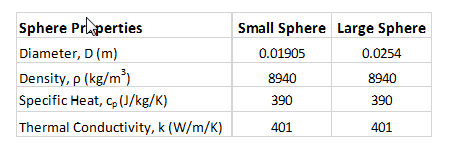
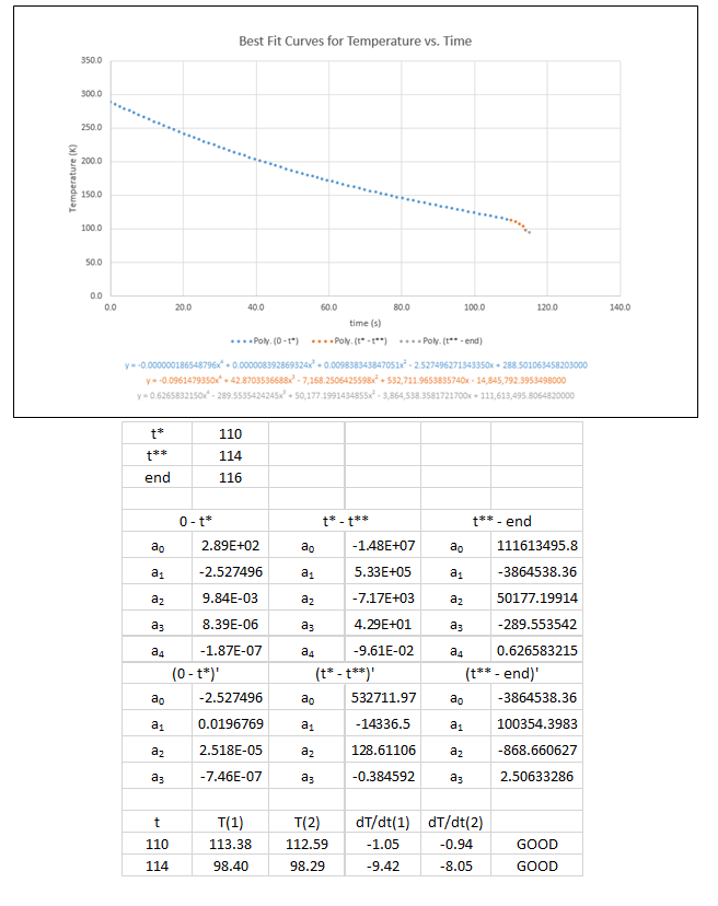
11. The following uncertainty calculations are performed on the following pages. Two sets of calculations were performed, one at t=110s and one at t=114s. The values were chosen because they are the locations of the minimum and maximum heat flux values respectively. The results are:
All uncertainties stem from initial uncertainties in sphere diameter and temperature readings, due to constraints in measurement ability. The results concerning the Biot number show that even with uncertainty considered, this experiment was well within the bounds of the lumped capacitance method (Bi < 0.1) even at the extremes. We can also see that, even with uncertainty taken into account in heat flux calculations, the accepted value remains outside of the range.
12.
a) Our results diminished the relative height of q’’s,max and the relative depth of q’’s,min. Effects on q’’s,max could have resulted in a temperature measurement reading that was too large during that period of time. Because at the point where q’’s is very high, the sphere temperature was changing very fast at that point. It is reasonable to think then, that measurements were taken with too much time between. Effects on q’’s,min may have been affected by differences in the outer and inner temperature reading on the sphere. A low q’’s would mean that the decrease in sphere temperature would be slow. The outer temperature is decreasing at a much slower rate than the inner temperature at that time. However, since the average temperature was used in data analysis, the slower decrease in temperature was offset by the still steadily decreasing inner temperature.
b) Difficulty arose in creating the boiling curve around the Leidenfrost point and at lower values of ΔTe. Problems in the boiling curve around the Leidenfrost point were already discussed in the previous comment. Discrepancies in the boiling curve at lower ΔTe were caused by a very unexpected stop in the further decrease of sphere temperature at T = -177°C or 96K. In theory, the temperature of the sphere should continue to decrease to the boiling point of nitrogen or 77K. We expected to stop the experiment, however at about 86K due to very slow temperature changes after that. The early leveling off of temperature may have been caused by large inaccuracies in temperature measurement at extremely low temperatures. It also may have been the result of faulty equipment calibration. Either way, it caused error in the boiling curve at around that point.
c) This experiment was much faster than the natural convection cooling experiment. In the natural convection, we were forced to wait upwards of half an hour for the plate to be cooled sufficiently. In this experiment, we finished each test in a matter of minutes. This is undoubtedly caused by the slower nature of natural convection. In natural convection the heat flux is very low while in a boiling situation, heat is being transferred at a high rate.
d) Peculiar behavior of the transient cooling rate mainly existed only near the Leidenfrost point, and again when the temperature of the sphere was very close to the boiling point of nitrogen.
e) The lumped capacitance method proved to be valid all the way though the experiment. Even at the Biot number extremes and considering uncertainty as well, the highest Biot number we could have experiences was Bi = .0277, which is still below the Bi < 0.1 requirement.
f) Our experimental maximum heat flux was smaller than the accepted value and the experimental minimum heat flux was larger than the accepted value. This would suggest that the data acquisition program used was unable to process large changes in temperature, either due to system faults or a measurement time interval that was too large.
g) The different flow regimes can be easily seen and identified on our plot of the boiling curve. I have done so on that figure.
Sphere Properties
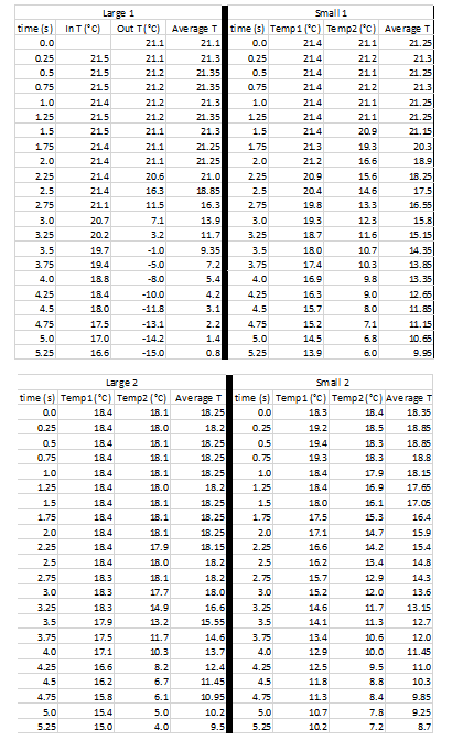
Original Test Results (sample from first 5.25 seconds)
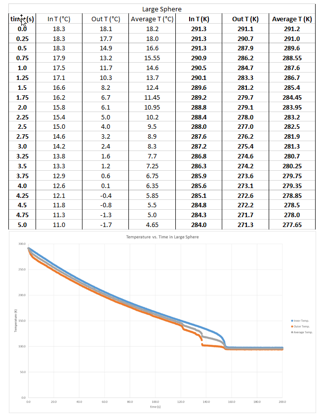
Pressure Gradient for Large Sphere (data sample from first 5 seconds and graph)
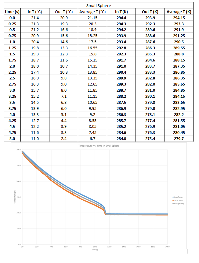
Pressure Gradient for Small Sphere (data sample from first 5 seconds and graph)
Best Fit Curve Approximations for Small Sphere Pressure Gradient
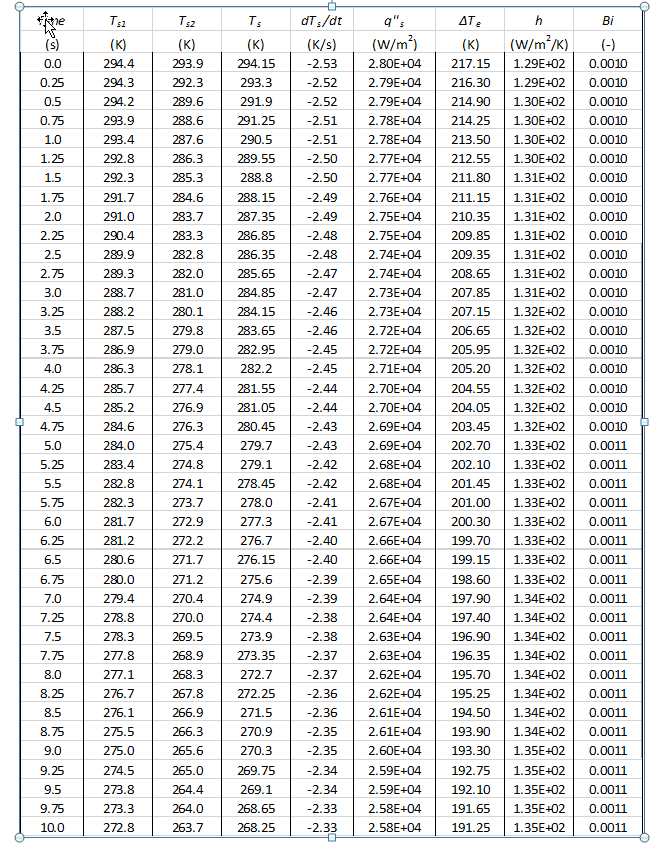
Small Sphere Data Calculations (sample from first 10 seconds)
Boiling Curve Production