Kinematic Linkage Systems: Analyzing Motion
Written by: Jeremy Stimack
Introduction
The analysis of the movement of a person has several powerful applications in determining the various biomechanical phenomena that occur within the body, such as joint motion or forces in the hip. Such information can provide valuable feedback in the research and development of medical devices that aid to remedy mechanical issues in affected individuals. Therefore, the objective of experimentation was to gain experience with a kinematic linkage system that is capable of measuring such motion and then apply it to quantify and analyze the walking gait of a subject.
Materials and Methods
The list of materials necessary to perform the entirety of Lab 6 include: five rotatory potentiometers; a tabletop linkage system; a goniometer; a kinematic linkage system with adjustable links and Velcro straps; a tape measure; adhesive tape; and a computer with LabVIEW software. Experimentation began by first calibrating the two rotary potentiometers of the tabletop linkage system. This was achieved by first taping a grid containing various dots of known distances from its origin onto the tabletop of the linkage system, ensuring that the origin of the grid aligned with the origin of the linkage system; any x-position offset was recorded using the tape measure. One team member then moved the pointer of the linkage system onto one of the dots on the calibration grid and measured the appropriate angles for each rotary potentiometer using the goniometer (see Figure 2). At the same location, the resistances of each potentiometer were then recorded using LabVIEW and saved in an Excel spreadsheet. This procedure was repeated for eight separate dots, and the calibration data was then used to determine resistance-angle relationships for either potentiometer, as depicted in Equation 1. The calibration grid was then removed from the tabletop and exchanged with a new grid containing two rows of capital letters. LabVIEW was then set to capture continuous data over twenty seconds, and the lengths of either arm of the linkage system were measured using the tape measure. Data capture was then initialized, and one lab member traced the first row of capital letters on the grid using the pointer of the linkage system; the resulting resistance data was then recorded and saved in an Excel spreadsheet. This procedure was repeated for the second row of the grid and for a “mystery word”, which was previously determined by the lab T.A. Once all data was recorded, a Matlab script applying Equations 2 – 3 was then written to calculate and plot the positions of the linkage pointer throughout data capture for the first and second row of the grid and for the “mystery word”.
Experimentation continued by then calibrating the rotary potentiometers of the kinematic linkage system. This was achieved by first laying the system down on a table and ensuring that the appropriate angles between each potentiometer and the arms of the linkage system were between 90 and 180 degrees (see Figure 3). Each angle was then measured using the goniometer, and the resistances of each potentiometer for these angles were then measured and saved in an Excel spreadsheet. This procedure was repeated for five trials, while altering the angles between each potentiometer and the respective arms of the linkage system for each trial, and the calibration data was then used to determine the resistance-angle relationships for each potentiometer, as depicted in Equation 4. The linkage system was then taken and strapped to the right leg of one team member using the Velcro straps, modifying any of the adjustable links as necessary to align the appropriate potentiometers with the hip, knee, and ankle joints, and the distances L0, L1, L2, and L3 (see Figure 3) were measured using the tape measure. The adhesive tape was then wrapped around the foot of the team member and the bottom of the linkage system, and the LabVIEW software was set to capture data continuously over ten seconds. Data capture was initialized, and the team member then walked two steps forward and stood still until data acquisition finished; the resulting resistance data for each potentiometer was then stored in an Excel spreadsheet. This procedure was repeated for two team members, with three trials each. The resulting resistances were then converted to angles by applying Equation 4, and then Equations 5 – 6 were applied to calculate the average velocities and accelerations of flexion and extension for each joint.
Equation 1
Pot 0 Angle = -0.1728×x_0 + 282.66; Pot 1 Angle= 0.1686×x_1 + 18.147; Where each angle is measured in degrees and x0 and x1 are the resistances of potentiometer 0 and potentiometer 1, respectively.
Equation 2
T_1=[■(cos(180-θ_1)&-sin(180-θ_1)&L_0@sin(180-θ_1)&cos(180-θ_1)&0@0&0&1)]; Where L0 is the length of the first linkage arm with x-axis offset and θ1 is the angle between L0 and the linkage pointer.
Equation 3
T_0=[■(cos(90-θ_0)&-sin(90-θ_0)&0@sin(90-θ_0)&cos(90-θ_0)&0@0&0&1)]; Where θ0 is the angle between the y-axis of the linkage coordinate system and the distance L0.
Equation 4
Pot 0 Angle= 0.1602×x_0 + 12.311; Pot 1 Angle=-0.1819×x_1 + 265.87; Pot 2 Angle=0.17×x_2 – 25.136; Where each angle is measured in degrees and x0, x1, and x2 are the resistances of potentiometer 0, potentiometer 1, and potentiometer 2, respectively.
Equation 5
w=∂θ/∂t; Where w is the angular velocity in rotations per second, θ is the flexion angle in degrees, and t is time in seconds.
Equation 6
α=∂w/∂t; Where α is the angular acceleration in meters per second per second, w is the angular velocity in rotations per second, and t is time in seconds.
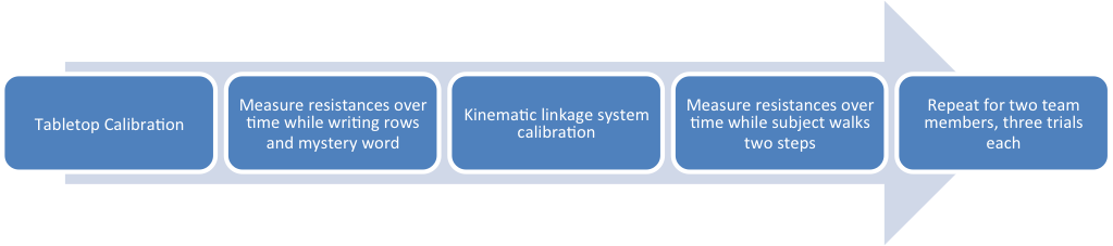
Figure 1 Visual depiction of the written methodology throughout experimentation in Lab 6.
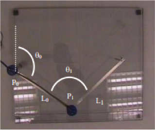
Figure 2: Visual depiction of the tabletop linkage system describing the angles and distances recorded throughout experimentation
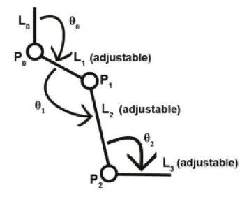
Figure 3: Visual depiction of the kinematic linkage system describing the angles and distances recorded throughout experimentation
Results
The resistance-angle relationships for each rotary potentiometer are listed in Equations 1 and 4. The measured x-axis offset for the calibration grid on the tabletop linkage system was 1.875 inches, with no offset in the y-axis, and the secret word was found to be “Goldy”. The average hip, knee, and ankle flexion angles for Subject 1 were determined to be 6.67, 43.67, and 10.8 degrees, respectively, and the average hip, knee, and ankle extension angles were determined to be 5.67, 15, and 18.3 degrees, respectively; the analysis of Subject 2’s gait produced similar results, with large differences existing only between the ankle extension and hip flexion angles. All calculated velocities and accelerations of flexion and extension for either subject were similar in magnitude, with large differences existing only between the accelerations of ankle extension and velocities of knee flexion (see Figures 5 – 7).
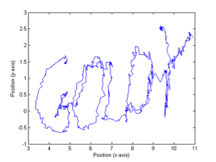
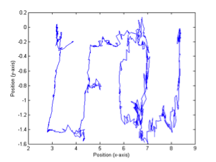
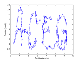
Figure 4: Resulting plots of the calculated pointer positions as the first, second, and mystery rows were traced.
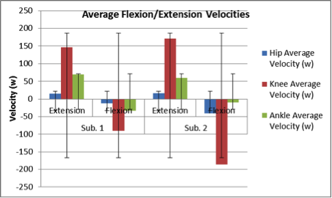
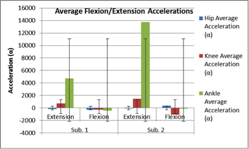
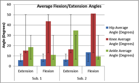
Figures 5-7: Graphical comparisons of the average extension/flexion angles, average velocities of extension/flexion, and average accelerations of extension/flexion for Subject 1 and Subject 2. Velocities were calculated through the application of Equation 5, and accelerations were calculated through the application of Equation 6.
Discussion
The difference between the measured and theoretical offset along the x-axis of the tabletop linkage system was relatively small; the transformation matrices predicted a value of 2.25 inches, while the measured offset was actually 1.875 inches. This discrepancy may have resulted from imperfect measuring of the x-axis offset with the tape measure, as well as rounding error when applying Equations 2 – 3. As depicted in Figure 4, the plotted images of the traced letters using the tabletop linkage system are correctly represented by the corresponding Matlab plots; however, they do not perfectly match the letters listed in Appendix C of the lab manual. This also may have been caused by rounding error when calculating the theoretical locations of the pointer, while imperfections in aligning the x-axis of the calibration grid with the x-axis of the tabletop linkage system may have resulted in incorrect resistance-angle relationships for the rotary potentiometers, leading to plotting error. Incorrect measurements of the positions of the dots on the calibration grid may further have resulted in slight variations between the plots. When analyzing the gaits of either subject during experimentation, it was evident that each walking pattern differed in stride length, leg flexion, and walking rate; one subject walked more quickly and with more motion around their hip, knee, and ankle joints, while the other subject walked with a higher pace. These differences are reflected in Figures 5 – 7. Possible error in measuring the kinematic linkage system’s calibration angles, however, may have resulted in incorrect resistance-angle relationships for its rotary potentiometers, leading to incorrect theoretical angle measurements and thus incorrect calculations of the velocities and accelerations of flexion/extension.
